Sut i gyfartaleddu ystod o ddata gan anwybyddu sero yn Excel?

Fel rheol, gall y swyddogaeth Gyfartalog eich helpu chi i gyfrifo cyfartaledd yr ystod gan gynnwys seroau yn Excel. Ond yma, rydych chi am eithrio'r seroau pan fyddwch chi'n cymhwyso'r swyddogaeth Gyfartalog. Sut allech chi anwybyddu sero mewn cyfrifiad cyfartalog?

Cyfartaledd ystod o ddata sy'n anwybyddu sero gyda fformiwla

Cyfartaledd / swm / cyfrif ystod o ddata gan anwybyddu sero gyda Kutools ar gyfer Excel      

Cyfartaledd ystod o ddata sy'n anwybyddu sero gyda fformiwla

Os ydych chi'n defnyddio Excel 2007/2010/2013, gall y swyddogaeth AVERAGEIF syml hon eich helpu i ddatrys y broblem hon yn gyflym ac yn hawdd.

1. Rhowch y fformiwla hon = AVERAGEIF (B2: B13, "<> 0") mewn cell wag ar wahân i'ch data, gweler y screenshot:

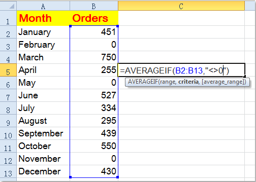
Nodyn: Yn y fformiwla uchod, B2: B13 yw'r data amrediad yr ydych am ei eithrio sero ar gyfartaledd, gallwch ei newid fel eich angen. Os oes celloedd gwag yn yr ystod, mae'r fformiwla hon hefyd yn cyfartaleddu'r data ac eithrio'r celloedd gwag.

2. Yna pwyswch Rhowch allweddol, a byddwch yn cael y canlyniad sydd wedi eithrio sero gwerthoedd. Gweler y screenshot:

Nodyn: Ni fydd y fformiwla hon yn dod i rym yn Excel 2003, os oes gennych Excel 2003, dylech gyfuno'r Swm ac Count swyddogaeth, cymhwyswch y fformiwla ganlynol: =SUM(B2:B13)/COUNTIF(B2:B13,">0").

Cyfartaledd / swm / cyfrif ystod o ddata gan anwybyddu sero gyda Kutools ar gyfer Excel

Os ydych chi am swm / cyfartaledd / cyfrif gan anwybyddu sero gelloedd, gallwch wneud cais Kutools ar gyfer Excel's Dewiswch Gelloedd Penodol cyfleustodau i ddewis celloedd nad ydynt yn sero, ac yna gweld canlyniad y cyfrifiad yn y Bar statws.

Ar ôl gosod am ddim Kutools ar gyfer Excel, gwnewch fel isod:

1. Dewiswch yr ystod rydych chi am ei chyfartalu, cliciwch Kutools > dewiswch > Dewiswch Gelloedd Penodol. Gweler y screenshot:

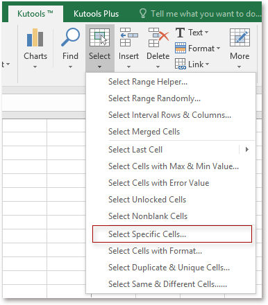
2. Yn y dialog popping, gwiriwch Cell dewis, ac yna dewis Dim yn cyfartal o'r gwymplen gyntaf i mewn Math penodol adran, ac ewch i'r blwch testun cywir i fynd i mewn 0. Gweler y screenshot:

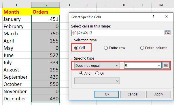
3. Cliciwch Ok, a dewiswyd pob cell sy'n fwy na 0, a gallwch weld y canlyniad cyfrif, swm, cyfrif cyfartalog yn y bar Statws. Gweler y screenshot:

Awgrym. Os ydych chi am gael treial am ddim o'r Dewiswch Cell Penodols swyddogaeth, os gwelwch yn dda ewch i lawrlwytho am ddim Kutools ar gyfer Excel yn gyntaf, ac yna ewch i gymhwyso'r llawdriniaeth yn ôl y camau uchod.

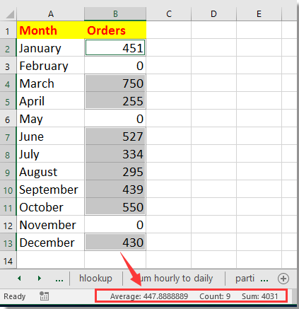
Mae data Cyfartaledd / Cyfrif / Swm yn anwybyddu seroau

Erthygl gysylltiedig:

Sut i gyfrifo gwerthoedd cyfartalog heb uchafswm a lleiaf yn Excel?

Offer Cynhyrchiant Swyddfa Gorau

🤖	Kutools AI Aide: Chwyldro dadansoddi data yn seiliedig ar: Cyflawniad Deallus   |  Cynhyrchu Cod  |  Creu Fformiwlâu Personol  |  Dadansoddi Data a Chynhyrchu Siartiau  |  Invoke Swyddogaethau Kutools...
	Nodweddion Poblogaidd: Darganfod, Amlygu neu Adnabod Dyblygiadau   |  Dileu Rhesi Gwag   |  Cyfuno Colofnau neu Gelloedd heb Colli Data   |   Rownd heb Fformiwla ...
	Super-edrych: VLookup Meini Prawf Lluosog  |   VLookup Gwerth Lluosog  |   VLookup Ar Draws Taflenni Lluosog   |   Edrych Niwlog ....
	Rhestr gwympo Uwch: Creu Rhestr Gollwng yn Gyflym   |  Rhestr Gollwng Dibynnol   |  Rhestr Gollwng Aml-ddewis ....
	Rheolwr Colofn: Ychwanegu Nifer Penodol o Golofnau  |  Symud Colofnau  |  Toglo Statws Gwelededd Colofnau Cudd  |  Cymharwch Ystodau a Cholofnau ...
	Nodweddion dan Sylw: Ffocws ar y Grid   |  Golwg Dylunio   |   Bar Fformiwla Mawr   |  Rheolwr Llyfr Gwaith a Thaflen   |  Llyfrgell Adnoddau (Testun Auto)   |  Dewiswr Dyddiad   |  Cyfuno Taflenni Gwaith   |  Amgryptio/Dadgryptio Celloedd   |  Anfon E-byst trwy Restr   |  Hidlo Super   |   Hidlo Arbennig (hidlo mewn print trwm/italig/strikethrough...) ...
	15 Set Offer Gorau:  12 Testun offer (Ychwanegu Testun, Dileu Cymeriadau,...)   |   50 + Siart Mathau (Siart Gantt,...)   |   40+ Ymarferol Fformiwlâu (Cyfrifwch oedran yn seiliedig ar ben-blwydd,...)   |   19 mewnosod offer (Mewnosod Cod QR, Mewnosod Llun o'r Llwybr,...)   |   12 Trosi offer (Rhifau i Eiriau, Trosi arian cyfred,...)   |   7 Uno a Hollti offer (Rhesi Cyfuno Uwch, Celloedd Hollt,...)   |   ... a mwy

Supercharge Eich Sgiliau Excel gyda Kutools ar gyfer Excel, a Phrofiad Effeithlonrwydd Fel Erioed Erioed. Kutools ar gyfer Excel Yn Cynnig Dros 300 o Nodweddion Uwch i Hybu Cynhyrchiant ac Arbed Amser.  Cliciwch Yma i Gael Y Nodwedd Sydd Ei Angen Y Mwyaf...

Read More ... Lawrlwythiad Am Ddim...

---

Mae Office Tab yn dod â rhyngwyneb Tabbed i Office, ac yn Gwneud Eich Gwaith yn Haws o lawer

• Galluogi golygu a darllen tabbed yn Word, Excel, PowerPoint, Cyhoeddwr, Mynediad, Visio a Phrosiect.
• Agor a chreu dogfennau lluosog mewn tabiau newydd o'r un ffenestr, yn hytrach nag mewn ffenestri newydd.
• Yn cynyddu eich cynhyrchiant 50%, ac yn lleihau cannoedd o gliciau llygoden i chi bob dydd!

Read More ... Lawrlwythiad Am Ddim...