Skip i'r prif gynnwys

Sut i drosi'r dyddiad i flwyddyn ariannol / chwarter / mis yn Excel?

Os oes gennych chi restr o ddyddiadau mewn taflen waith, a'ch bod chi am gadarnhau blwyddyn ariannol / chwarter / mis y dyddiadau hyn yn gyflym, gallwch chi ddarllen y tiwtorial hwn, rwy'n credu efallai y byddwch chi'n dod o hyd i'r ateb.

Dyddiad trosi i flwyddyn ariannol

Trosi dyddiad i chwarter cyllidol

Trosi dyddiad i fis cyllidol


swigen dde glas saeth Dyddiad trosi i flwyddyn ariannol

1. Dewiswch gell, a theipiwch rif mis cychwynnol y flwyddyn ariannol, yma, mae blwyddyn ariannol fy nghwmni yn dechrau o Orffennaf 1af, ac rwy'n teipio 7. Gweler y screenshot:
doc-trosi-cyllidol-blwyddyn-1

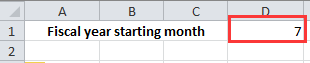
2. Yna gallwch chi deipio'r fformiwla hon =YEAR(DATE(YEAR(A4),MONTH(A4)+($D$1-1),1)) i mewn i gell wrth ymyl eich dyddiadau, yna llusgwch yr handlen llenwi i ystod sydd ei hangen arnoch chi.doc-trosi-cyllidol-blwyddyn-2

Tip: Yn y fformiwla uchod, mae A4 yn nodi'r gell ddyddiad, ac mae D1 yn nodi'r mis y mae'r flwyddyn ariannol yn dechrau ynddo.


swigen dde glas saeth Trosi dyddiad i chwarter cyllidol

Os ydych chi am drosi'r dyddiad yn chwarter cyllidol, gallwch chi wneud fel y rhain:

1. Yn gyntaf, mae angen i chi wneud tabl fel y dangosir isod. Yn rhestr y rhes gyntaf bob mis o flwyddyn, yna yn yr ail reng, teipiwch y rhif chwarter cyllidol cymharol i bob mis. Gweler y screenshot:
doc-trosi-cyllidol-blwyddyn-3

2. Yna mewn cell wrth ymyl eich colofn dyddiad, a theipiwch y fformiwla hon = DEWIS (MIS (A6), 3,3,3,4,4,4,1,1,1,2,2,2) i mewn iddo, yna llusgwch yr handlen llenwi i ystod sydd ei hangen arnoch chi.doc-trosi-cyllidol-blwyddyn-4

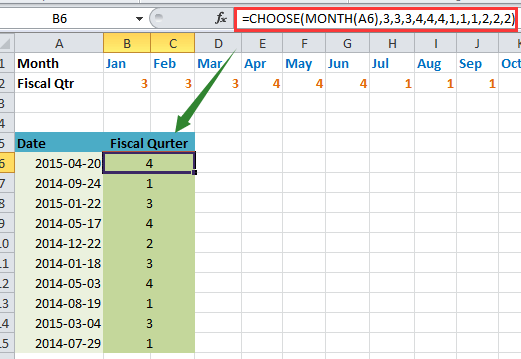
Tip: Yn y fformiwla uchod, A6 yw'r gell ddyddiad, a'r gyfres rifau 3,3,3 ... yw'r gyfres chwarter cyllidol y gwnaethoch ei theipio yng ngham 1.


swigen dde glas saeth Trosi dyddiad i fis cyllidol

I drosi'r dyddiad yn fis cyllidol, mae angen i chi wneud tabl yn gyntaf hefyd.

1. Yn rhestr y rhes gyntaf trwy'r mis o flwyddyn, yna yn yr ail reng, teipiwch rif y mis cyllidol cymharol i bob mis. Gweler y screenshot:doc-trosi-cyllidol-blwyddyn-5

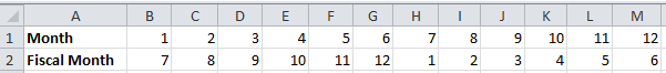
2. Yna mewn cell wrth ymyl y golofn, teipiwch y fformiwla hon = DEWIS (MIS (A6), 7,8,9,10,11,12,1,2,3,4,5,6) i mewn iddo, a llusgwch yr handlen llenwi i'ch ystod angenrheidiol gyda'r fformiwla hon. doc-trosi-cyllidol-blwyddyn-6

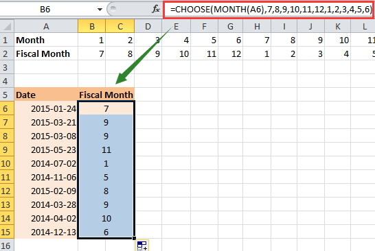
Tip: Yn y fformiwla uchod, A6 yw'r gell ddyddiad, a'r gyfres rifau 7,8,9 ... yw'r gyfres rhifau mis cyllidol rydych chi'n ei theipio yng ngham 1.


Trosi dyddiad ansafonol yn gyflym i fformatio dyddiad safonol (mm / dd / bbbb)

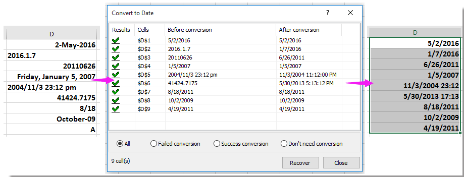
Mewn rhai adegau, efallai y byddwch yn derbyn setiau gwaith gyda nifer o ddyddiadau ansafonol, ac i drosi pob un ohonynt i'r fformatio dyddiad safonol gan fod mm / dd / bbbb yn drafferthus i chi. Yma Kutools ar gyfer Excel's Cydgyfeirio hyd yn hyn yn gallu trosi'r dyddiadau ansafonol hyn yn gyflym i'r fformatio dyddiad safonol gydag un clic.  Cliciwch i gael treial llawn am ddim mewn 30 diwrnod!
dyddiad trosi doc
 
Kutools ar gyfer Excel: gyda mwy na 300 o ychwanegion Excel defnyddiol, am ddim i geisio heb unrhyw gyfyngiad mewn 30 diwrnod.

Offer Cynhyrchiant Swyddfa Gorau

🤖 Kutools AI Aide: Chwyldro dadansoddi data yn seiliedig ar: Cyflawniad Deallus   |  Cynhyrchu Cod  |  Creu Fformiwlâu Personol  |  Dadansoddi Data a Chynhyrchu Siartiau  |  Invoke Swyddogaethau Kutools...
Nodweddion Poblogaidd: Darganfod, Amlygu neu Adnabod Dyblygiadau   |  Dileu Rhesi Gwag   |  Cyfuno Colofnau neu Gelloedd heb Colli Data   |   Rownd heb Fformiwla ...
Super-edrych: VLookup Meini Prawf Lluosog    VLookup Gwerth Lluosog  |   VLookup Ar Draws Taflenni Lluosog   |   Edrych Niwlog ....
Rhestr gwympo Uwch: Creu Rhestr Gollwng yn Gyflym   |  Rhestr Gollwng Dibynnol   |  Rhestr Gollwng Aml-ddewis ....
Rheolwr Colofn: Ychwanegu Nifer Penodol o Golofnau  |  Symud Colofnau  |  Toglo Statws Gwelededd Colofnau Cudd  |  Cymharwch Ystodau a Cholofnau ...
Nodweddion dan Sylw: Ffocws ar y Grid   |  Golwg Dylunio   |   Bar Fformiwla Mawr    Rheolwr Llyfr Gwaith a Thaflen   |  Llyfrgell Adnoddau (Testun Auto)   |  Dewiswr Dyddiad   |  Cyfuno Taflenni Gwaith   |  Amgryptio/Dadgryptio Celloedd    Anfon E-byst trwy Restr   |  Hidlo Super   |   Hidlo Arbennig (hidlo mewn print trwm/italig/strikethrough...) ...
15 Set Offer Gorau12 Testun offer (Ychwanegu Testun, Dileu Cymeriadau,...)   |   50 + Siart Mathau (Siart Gantt,...)   |   40+ Ymarferol Fformiwlâu (Cyfrifwch oedran yn seiliedig ar ben-blwydd,...)   |   19 mewnosod offer (Mewnosod Cod QR, Mewnosod Llun o'r Llwybr,...)   |   12 Trosi offer (Rhifau i Eiriau, Trosi arian cyfred,...)   |   7 Uno a Hollti offer (Rhesi Cyfuno Uwch, Celloedd Hollt,...)   |   ... a mwy

Supercharge Eich Sgiliau Excel gyda Kutools ar gyfer Excel, a Phrofiad Effeithlonrwydd Fel Erioed Erioed. Kutools ar gyfer Excel Yn Cynnig Dros 300 o Nodweddion Uwch i Hybu Cynhyrchiant ac Arbed Amser.  Cliciwch Yma i Gael Y Nodwedd Sydd Ei Angen Y Mwyaf...

Disgrifiad


Mae Office Tab yn dod â rhyngwyneb Tabbed i Office, ac yn Gwneud Eich Gwaith yn Haws o lawer

  • Galluogi golygu a darllen tabbed yn Word, Excel, PowerPoint, Cyhoeddwr, Mynediad, Visio a Phrosiect.
  • Agor a chreu dogfennau lluosog mewn tabiau newydd o'r un ffenestr, yn hytrach nag mewn ffenestri newydd.
  • Yn cynyddu eich cynhyrchiant 50%, ac yn lleihau cannoedd o gliciau llygoden i chi bob dydd!
Comments (27)
No ratings yet. Be the first to rate!
This comment was minimized by the moderator on the site
How to set If formula is target is month i.e 07.2023 , 08.2022 ...
This comment was minimized by the moderator on the site
For Find in FY Year by month
This comment was minimized by the moderator on the site
Hi, I would like to get an OUTPUT as a Date(10/11/2022) in Colum F, from a Fiscal Year (2023) in column A and Month(11) in Colum D. As my fiscal Year starts from November and Ends in October.

Appreciate your help to find a formula in Excel. Thank
This comment was minimized by the moderator on the site
=IF(MONTH(EOMONTH(B4,0))>3,

YEAR(B4)&"-"&RIGHT(YEAR(B4)+1,2),

YEAR(B4)-1&"-"&RIGHT(YEAR(B4),2))
https://excelforfinance1.blogspot.com/2021/05/excel-formula-to-get-financial-year.html </div>;
This comment was minimized by the moderator on the site
Just check this

=IF(MONTH(I8)>3,"FY"&YEAR(I8)&"-"&YEAR(I8)+1,IF(MONTH(I8)<=3,"FY"&YEAR(I8)-1&"-"&YEAR(I8)))

Assume the target is in I8 cell with a date of 8/23/2011 , the out put will be FY2011-2012

Sathish
This comment was minimized by the moderator on the site
worked well...thank you.
This comment was minimized by the moderator on the site
Just check this
=IF(MONTH(I8)>3,"FY"&YEAR(I8)&"-"&YEAR(I8)+1,IF(MONTH(I8)<=3,"FY"&YEAR(I8)-1&"-"&YEAR(I8)))

Assume the target is in I8 cell with a date of 8/23/2011 , the out put will be <span style="letter-spacing: 0.2px; color: inherit; font-family: inherit; font-style: inherit; font-variant-ligatures: inherit; font-variant-caps: inherit; font-weight: inherit;"> </span>
Sathish
This comment was minimized by the moderator on the site
If anyone is looking for a formula to figure out what fiscal/policy year an payment/event happened, even if that fiscal year/policy doesn't start on the first of the month I came up with this.

=YEAR(A4)+((MONTH(A4)>=MONTH($D$1)+(DAY(A4)<Day($D$1)))-1)

D1 in this has to be a full date 01/06/2019 for example.

Also surely a cheeky Vlookup is a better way of doing the quarter formula

=Vlookup(Month(A6),etc.)
This comment was minimized by the moderator on the site
"=Vlookup(Month(A6),etc.)" It's so simple, yet so elegant... not sure why I didn't think of this but this was a huge find. Thank you!
This comment was minimized by the moderator on the site
I came up with a self contained choose() to calculate the fiscal year that doesn't need to use an external cell as an input.
.
Fiscal Year EndCalculation
="June 30, " & (YEAR(E2) +CHOOSE(MONTH(E2),0,0,0,0,0,0,1,1,1,1,1,1))
. * The first part is just a text string
. * & concatenates the first part to the second part which calculatesthe appropriate year.
. * Year(e2) extracts the year number from the date in column E
. * Choose() looks at the month number from that same date.
. For months Jan through June itretrieves the value 0,
. For months July thru Dec itretrieves value 1.
. The retrieved value is added to theyear extracted to give the appropriate year end
“June 30, 2020”.

This is on the assumption that a company is not likely to be changing it's year end. Doesn't work if the sheet is being used for multiple companies with different year ends ...
This comment was minimized by the moderator on the site
Please correct the fiscal-year formula you give above! It does not work unless the fiscal year begins with month 7. This formula will work just fine:

=YEAR(DATE(YEAR(A4),MONTH(A4)+12-($D$1-1),1))

But it is still way more complex than it needs to be. Use Michael's formula (but correct his typo):

=YEAR(A4)+(MONTH(A4)>=$D$1)
This comment was minimized by the moderator on the site
IF YOU WANT TO FIND FISCAL YEAR IN INDIA....
WRITE EXCEL QUERY AS BELOW


=(YEAR(DATE)+(MONTH(DATE)>=4))-1
This comment was minimized by the moderator on the site
You can use below formulae:


Here Col K2 is our date column which is to be converted in format 20XX-XY (e.g. 2017-18).

=IF(MONTH(K2)<4,TEXT(DATE(YEAR(K2)-1,MONTH(K2),DAY(K2)),"YYYY-")&TEXT(DATE(YEAR(K2),MONTH(K2),DAY(K2)),"YY"),TEXT(DATE(YEAR(K2),MONTH(K2),DAY(K2)),"YYYY-")&TEXT(DATE(YEAR(K2)+1,MONTH(K2),DAY(K2)),"YY"))
This comment was minimized by the moderator on the site
You can also use below formula for the same condition :


=IF(MONTH(K2)<4,YEAR(K2)-1&"-"&TEXT(K2,"YY"),YEAR(K2)&"-"&TEXT(K2,"YY")+1)
This comment was minimized by the moderator on the site
Thank you!!
This comment was minimized by the moderator on the site
What a legend. Thank you!
This comment was minimized by the moderator on the site
thank you
There are no comments posted here yet
Load More
Please leave your comments in English
Posting as Guest
×
Rate this post:
0   Characters
Suggested Locations