Sut i gyfartaledd 5 gwerth olaf colofn wrth i rifau newydd ddod i mewn?
Yn Excel, gallwch chi gyfrifo cyfartaledd y 5 gwerth diwethaf yn gyflym mewn colofn gyda'r swyddogaeth Gyfartalog, ond, o bryd i'w gilydd, mae angen i chi nodi rhifau newydd y tu ôl i'ch data gwreiddiol, ac rydych chi am i'r canlyniad cyfartalog gael ei newid yn awtomatig fel y data newydd sy'n mynd i mewn. Hynny yw, hoffech chi gael y cyfartaledd bob amser yn adlewyrchu 5 rhif olaf eich rhestr ddata, hyd yn oed pan fyddwch chi'n ychwanegu rhifau nawr ac yn y man.
5 gwerth olaf colofn ar gyfartaledd fel rhifau newydd sy'n mynd i mewn gyda fformwlâu
 5 gwerth olaf colofn ar gyfartaledd fel rhifau newydd sy'n mynd i mewn gyda fformwlâu
Efallai y bydd y fformwlâu arae canlynol yn eich helpu i ddatrys y broblem hon, gwnewch fel a ganlyn:
Rhowch y fformiwla hon mewn cell wag:
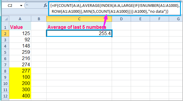
=IF(COUNT(A:A),AVERAGE(INDEX(A:A,LARGE(IF(ISNUMBER(A1:A10000),ROW(A1:A10000)),MIN(5,COUNT(A1:A10000)))):A10000),"no data") (A: A yw'r golofn sy'n cynnwys y data a ddefnyddiwyd gennych, A1: A10000 yn ystod ddeinamig, gallwch ei ehangu cyhyd â'ch angen, a'r rhif 5 yn nodi'r gwerth n olaf.), ac yna pwyswch Ctrl + Shift + Enter allweddi gyda'i gilydd i gael cyfartaledd y 5 rhif olaf. Gweler y screenshot:

Ac yn awr, pan fyddwch yn mewnbynnu rhifau newydd y tu ôl i'r data gwreiddiol, bydd y cyfartaledd yn cael ei newid hefyd, gweler y screenshot:
Nodyn: Os yw'r golofn o gelloedd yn cynnwys 0 gwerth, rydych chi am eithrio'r 0 gwerth o'ch 5 rhif diwethaf, ni fydd y fformiwla uchod yn gweithio, yma, gallaf gyflwyno fformiwla arae arall i chi i gael cyfartaledd y 5 gwerth olaf nad ydynt yn sero. , nodwch y fformiwla hon:
=AVERAGE(SUBTOTAL(9,OFFSET(A1:A10000,LARGE(IF(A1:A10000>0,ROW(A1:A10000)-MIN(ROW(A1:A10000))),ROW(INDIRECT("1:5"))),0,1))), ac yna'r wasg Ctrl + Shift + Enter allweddi i gael y canlyniad sydd ei angen arnoch, gweler y screenshot:

Erthyglau cysylltiedig:
Sut i gyfartaledd pob 5 rhes neu golofn yn Excel?
Sut i gyfartaledd gwerthoedd 3 uchaf neu isaf yn Excel?
Offer Cynhyrchiant Swyddfa Gorau
Supercharge Eich Sgiliau Excel gyda Kutools ar gyfer Excel, a Phrofiad Effeithlonrwydd Fel Erioed Erioed. Kutools ar gyfer Excel Yn Cynnig Dros 300 o Nodweddion Uwch i Hybu Cynhyrchiant ac Arbed Amser. Cliciwch Yma i Gael Y Nodwedd Sydd Ei Angen Y Mwyaf...
")
Mae Office Tab yn dod â rhyngwyneb Tabbed i Office, ac yn Gwneud Eich Gwaith yn Haws o lawer
- Galluogi golygu a darllen tabbed yn Word, Excel, PowerPoint, Cyhoeddwr, Mynediad, Visio a Phrosiect.
- Agor a chreu dogfennau lluosog mewn tabiau newydd o'r un ffenestr, yn hytrach nag mewn ffenestri newydd.
- Yn cynyddu eich cynhyrchiant 50%, ac yn lleihau cannoedd o gliciau llygoden i chi bob dydd!
")