Skip i'r prif gynnwys

Sut i edrych ar gyfeiriad cell gwerth a dychwelyd yn Excel?

Yn gyffredinol, byddwch chi'n cael gwerth y gell pan fyddwch chi'n defnyddio fformiwla i chwilio am werth yn Excel. Ond yma, byddaf yn cyflwyno rhai fformiwlâu i edrych ar werth a dychwelyd y cyfeiriad celloedd cymharol.

Edrychwch ar gyfeiriad cell gwerth a dychwelyd gyda fformiwla


swigen dde glas saeth Edrychwch ar gyfeiriad cell gwerth a dychwelyd gyda fformiwla

I edrych ar werth a dychwelyd cyfeiriad cell cyfatebol yn lle gwerth celloedd yn Excel, gallwch ddefnyddio'r fformwlâu isod.

Fformiwla 1 I ddychwelyd cyfeirnod absoliwt y gell

Er enghraifft, mae gennych ystod o ddata fel y dangosir isod screenshot, ac rydych chi am edrych ar gynnyrch AA a dychwelyd y cyfeirnod absoliwt cymharol celloedd.
doc-vlookup-dychwelyd-gell-cyfeiriad-1

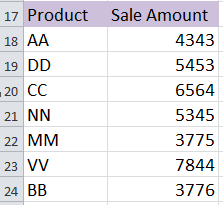
1. Dewiswch gell a theipiwch AA ynddo, dyma fi'n teipio AA i mewn i gell A26. Gweler y screenshot:
doc-vlookup-dychwelyd-gell-cyfeiriad-2

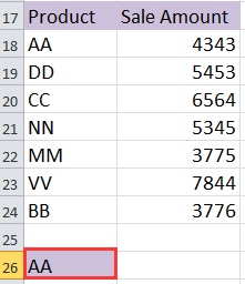
2. Yna teipiwch y fformiwla hon =CELL("address",INDEX($A$18:$A$24,MATCH(A26,$A$18:$A$24,1))) yn y gell ger cell A26 (y gell y gwnaethoch chi deipio AA), yna pwyswch Shift + Ctrl + Enter allweddi a byddwch yn cael y cyfeirnod celloedd cymharol. Gweler y screenshot:
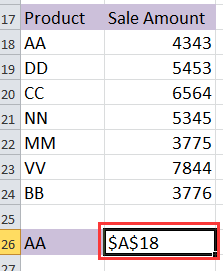
doc-vlookup-dychwelyd-gell-cyfeiriad-3

Tip:

1. Yn y fformiwla uchod, A18: A24 yw'r amrediad colofn y mae eich gwerth edrych ynddo, A26 yw'r gwerth edrych.

2. Dim ond y cyfeiriad cell cymharol cyntaf hwn sy'n cyfateb i'r gwerth edrych sy'n gallu dod o hyd i'r fformiwla hon.

Fformiwla 2 I ddychwelyd rhif rhes gwerth y gell yn y tabl

Er enghraifft, mae gennych ddata fel y dangosir isod, rydych chi am edrych ar gynnyrch BB a dychwelyd ei holl gyfeiriadau celloedd yn y tabl.
doc-vlookup-dychwelyd-gell-cyfeiriad-4

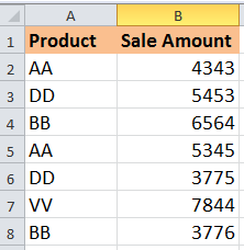
1. Teipiwch BB i mewn i gell, dyma fi'n teipio BB i mewn i gell A10. Gweler y screenshot:
doc-vlookup-dychwelyd-gell-cyfeiriad-5

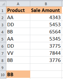
2. Yn y gell ger y gell A10 (y gell y gwnaethoch chi deipio BB), teipiwch y fformiwla hon =SMALL(IF($A$10=$A$2:$A$8, ROW($A$2:$A$8)-ROW($A$2)+1), ROW(1:1)), a'r wasg Shift + Ctrl + Enter allweddi, yna llusgwch y handlen llenwi auto i lawr i gymhwyso'r fformiwla hon nes ei bod yn ymddangos #NUM !. gweler y screenshot:
doc-vlookup-dychwelyd-gell-cyfeiriad-6

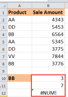
3. Yna gallwch chi ddileu #NUM !. Gweler y screenshot:
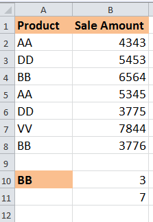
doc-vlookup-dychwelyd-gell-cyfeiriad-7

Awgrym:

1. Yn y fformiwla hon, mae A10 yn nodi'r gwerth edrych, ac A2: A8 yw'r amrediad colofn y mae eich gwerth edrych ynddo.

2. Gyda'r fformiwla hon, dim ond rhifau rhes y celloedd cymharol y gallwch eu cael yn y tabl ac eithrio pennawd y bwrdd.

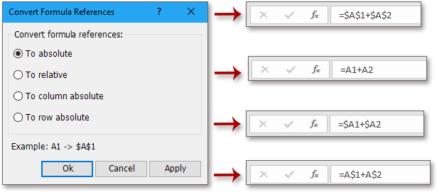
Swp Trosi cyfeirnod fformiwla at absoliwt, cymharol, colofn absoliwt neu Row Absolute

Weithiau, efallai yr hoffech chi drosi'r cyfeirnod fformiwla yn absoliwt, ond yn Excel, dim ond trosi gall y cyfeiriadau fesul un y gall gwastraffu amser tra bod cannoedd o fformiwlâu. Mae'r Trosi Cyfeirnod o Kutools ar gyfer Excel gall swp drosi'r cyfeiriadau mewn celloedd dethol i gymharol, absoliwt ag sydd ei angen arnoch.   Cliciwch ar gyfer treial llawn sylw 30 diwrnod am ddim!
doc kutools trosi cyfeirnod 1
 
Kutools ar gyfer Excel: gyda mwy na 300 o ychwanegion Excel defnyddiol, am ddim i geisio heb unrhyw gyfyngiad mewn 30 diwrnod.

Erthyglau Perthynas

Offer Cynhyrchiant Swyddfa Gorau

🤖 Kutools AI Aide: Chwyldro dadansoddi data yn seiliedig ar: Cyflawniad Deallus   |  Cynhyrchu Cod  |  Creu Fformiwlâu Personol  |  Dadansoddi Data a Chynhyrchu Siartiau  |  Invoke Swyddogaethau Kutools...
Nodweddion Poblogaidd: Darganfod, Amlygu neu Adnabod Dyblygiadau   |  Dileu Rhesi Gwag   |  Cyfuno Colofnau neu Gelloedd heb Colli Data   |   Rownd heb Fformiwla ...
Super-edrych: VLookup Meini Prawf Lluosog    VLookup Gwerth Lluosog  |   VLookup Ar Draws Taflenni Lluosog   |   Edrych Niwlog ....
Rhestr gwympo Uwch: Creu Rhestr Gollwng yn Gyflym   |  Rhestr Gollwng Dibynnol   |  Rhestr Gollwng Aml-ddewis ....
Rheolwr Colofn: Ychwanegu Nifer Penodol o Golofnau  |  Symud Colofnau  |  Toglo Statws Gwelededd Colofnau Cudd  |  Cymharwch Ystodau a Cholofnau ...
Nodweddion dan Sylw: Ffocws ar y Grid   |  Golwg Dylunio   |   Bar Fformiwla Mawr    Rheolwr Llyfr Gwaith a Thaflen   |  Llyfrgell Adnoddau (Testun Auto)   |  Dewiswr Dyddiad   |  Cyfuno Taflenni Gwaith   |  Amgryptio/Dadgryptio Celloedd    Anfon E-byst trwy Restr   |  Hidlo Super   |   Hidlo Arbennig (hidlo mewn print trwm/italig/strikethrough...) ...
15 Set Offer Gorau12 Testun offer (Ychwanegu Testun, Dileu Cymeriadau,...)   |   50 + Siart Mathau (Siart Gantt,...)   |   40+ Ymarferol Fformiwlâu (Cyfrifwch oedran yn seiliedig ar ben-blwydd,...)   |   19 mewnosod offer (Mewnosod Cod QR, Mewnosod Llun o'r Llwybr,...)   |   12 Trosi offer (Rhifau i Eiriau, Trosi arian cyfred,...)   |   7 Uno a Hollti offer (Rhesi Cyfuno Uwch, Celloedd Hollt,...)   |   ... a mwy

Supercharge Eich Sgiliau Excel gyda Kutools ar gyfer Excel, a Phrofiad Effeithlonrwydd Fel Erioed Erioed. Kutools ar gyfer Excel Yn Cynnig Dros 300 o Nodweddion Uwch i Hybu Cynhyrchiant ac Arbed Amser.  Cliciwch Yma i Gael Y Nodwedd Sydd Ei Angen Y Mwyaf...

Disgrifiad


Mae Office Tab yn dod â rhyngwyneb Tabbed i Office, ac yn Gwneud Eich Gwaith yn Haws o lawer

  • Galluogi golygu a darllen tabbed yn Word, Excel, PowerPoint, Cyhoeddwr, Mynediad, Visio a Phrosiect.
  • Agor a chreu dogfennau lluosog mewn tabiau newydd o'r un ffenestr, yn hytrach nag mewn ffenestri newydd.
  • Yn cynyddu eich cynhyrchiant 50%, ac yn lleihau cannoedd o gliciau llygoden i chi bob dydd!
Comments (26)
No ratings yet. Be the first to rate!
This comment was minimized by the moderator on the site
HI. In sheet 1, I need a certain value present in sheet 2 to be returned. Therefore, in column A of sheet 2, first of all I have to look for a cell containing a specific text (all the cells in column A contain a different text) . From this cell I have to go two rows down and 33 columns to the right of this specific text cell. This is the sheet 2 cell containing my value to import into sheet 1. How can I do this? Could you please help me ? Thank you very much
This comment was minimized by the moderator on the site
Die Formel =CELL("address",INDEX($A$18:$A$24,MATCH(A26,$A$18:$A$24,1))) ist genau das, was ich suche!!!

Tipp 2. "Diese Formel kann nur die erste relative Zellenadresse finden, die dem Suchwert entspricht." beschreibt genau mein Problem: ich benötige die letzte relative Zellenadresse, die dem Suchwert entspricht. Ist das machbar?

Danke und Gruß
Micha
This comment was minimized by the moderator on the site
Hi, Damich, below formula will lookup value from bottom, and return the relative cell address:
=CELL("address",INDEX($A$1:$A$7,MATCH(2,1/($A$1:$A$7=A10),1)))
This comment was minimized by the moderator on the site
If my data is in any sheet of the workbook whether in sheet 1, or sheet 2, or sheet 3, how can I find the cell address of this data with the help of formula.

pls advise.....
This comment was minimized by the moderator on the site
Hi, you can add the sheet name in the formula: =CELL("address",INDEX(Sheet1!$A$18:$A$24,MATCH(A26,Sheet1!$A$18:$A$24,1))), Sheet1 is the sheet name that contains your data.
This comment was minimized by the moderator on the site
감사합니다.

다만
=CELL("address",INDEX($A$18:$A$24,MATCH(A26,$A$18:$A$24,1)))
->
=CELL("address",INDEX($A$18:$A$24,MATCH(A26,$A$18:$A$24,0)))
MATCH함수 마지막에 1이 아닌 0을 기입해야
AA가 아닌 BB의 위치도 반환이 되는 것 같아요.

훌륭한 설명 감사합니다.

큰 도움이 됬어요.
This comment was minimized by the moderator on the site
Is there any formula for this case below to summarize following Alphabet of results? For example: which numbers belong to A/B/..
A=1; E=42; D=64; C=32; B=20; D=9; A=10; B=22; D=45; C=21; E=30; E=59; A=33; D=23; C=11; B=25; B=49; D=6; D=99; E=89; A=70; D=27; B=4; C=47; D=68; E=62; A=57; A=86; B=91; D=93; C=18; D=12; A=55; D=50; ect.
==> expect for result: A=1;10;33;70;57;86;55
My email: thanks so much
This comment was minimized by the moderator on the site
Can we modify the formula =CELL("address",INDEX($A$18:$A$24,MATCH(A26,$A$18:$A$24,1))) to get all the cell addresses which contains a specific text string like an array formula
This comment was minimized by the moderator on the site
Can we modify the formula =CELL("address",INDEX($A$18:$A$24,MATCH(A26,$A$18:$A$24,1))) to get all the cell addresses which contains a specific text string
This comment was minimized by the moderator on the site
Have no idea.
This comment was minimized by the moderator on the site
=CELL("address",INDEX($A$18:$A$24,MATCH(A26,$A$18:$A$24,1))) excellent this function for me but i want cell reference address across multiple sheets.
This comment was minimized by the moderator on the site
Try to add the sheet name in the formula like =CELL("address",INDEX(Sheet1!$A$18:$A$24,MATCH(Sheet2!A26,Sheet1!$A$18:$A$24,1))).
This comment was minimized by the moderator on the site
I would like to lookup the address of the max value in column.
This comment was minimized by the moderator on the site
Hi, sorry to repy so late, if you also need the answer, this tutorial will help you: How To Find Address Of Cell With Max Or Min Value In Excel?
This comment was minimized by the moderator on the site
Hi Master,

What formula for search "value" belong to which sheet , address in excel file with 100 worksheet tab
There are no comments posted here yet
Load More
Please leave your comments in English
Posting as Guest
×
Rate this post:
0   Characters
Suggested Locations