Skip i'r prif gynnwys

Sut i wylio a symio gemau mewn rhesi neu golofnau yn Excel?

Mae defnyddio swyddogaeth gwylio a swm yn eich helpu i ddarganfod y meini prawf penodedig yn gyflym a chrynhoi'r gwerthoedd cyfatebol ar yr un pryd. Yn yr erthygl hon, rydyn ni'n mynd i ddangos dau ddull i chi wylio a chrynhoi'r gwerthoedd cyntaf neu'r holl werthoedd cyfatebol mewn rhesi neu golofnau yn Excel.

Mae Vlookup a sum yn cyfateb yn olynol neu resi lluosog gyda fformwlâu
Gemau gwylio a swm mewn colofn gyda fformwlâu
Hawdd gwylio a chyfateb gemau mewn rhesi neu golofnau gydag offeryn anhygoel

Mwy o sesiynau tiwtorial ar gyfer VLOOKUP ...


Mae Vlookup a sum yn cyfateb yn olynol neu resi lluosog gyda fformwlâu

Gall y fformwlâu yn yr adran hon helpu i grynhoi'r gwerthoedd cyntaf neu'r holl werthoedd cyfatebol yn olynol neu resi lluosog yn seiliedig ar feini prawf penodol yn Excel. Gwnewch fel a ganlyn.

Vlookup a swm y gwerth cyfatebol cyntaf yn olynol

Gan dybio bod gennych chi fwrdd ffrwythau fel y dangosir y llun isod, ac mae angen i chi edrych ar yr Afal cyntaf yn y tabl ac yna crynhoi'r holl werthoedd cyfatebol yn yr un rhes. I gyflawni hyn, gwnewch fel a ganlyn.

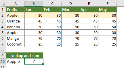
1. Dewiswch gell wag i allbwn y canlyniad, dyma fi'n dewis cell B10. Copïwch y fformiwla isod i mewn iddi a gwasgwch y Ctrl + Symud + Rhowch allweddi i gael y canlyniad.

=SUM(VLOOKUP(A10, $A$2:$F$7, {2,3,4,5,6}, FALSE))

Nodiadau:

  • A10 yw'r gell sy'n cynnwys y gwerth rydych chi'n edrych amdano;
  • $ A $ 2: $ F $ 7 yw ystod y tabl data (heb benawdau) sy'n cynnwys y gwerth edrych a'r gwerthoedd cyfatebol;
  • Mae nifer {2,3,4,5,6} yn cynrychioli bod y colofnau gwerth canlyniad yn dechrau gyda'r ail golofn ac yn gorffen gyda chweched golofn y tabl. Os yw nifer y colofnau canlyniad yn fwy na 6, newidiwch {2,3,4,5,6} i {2,3,4,5,6,7,8,9….}.
Vlookup a swm yr holl werthoedd cyfatebol mewn rhesi lluosog

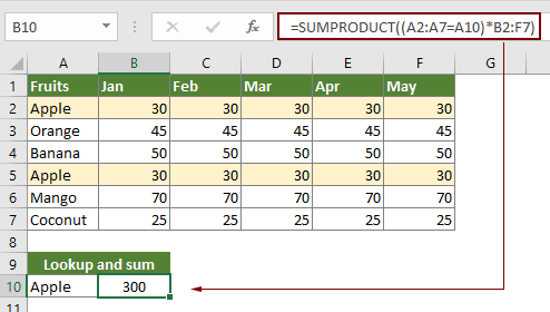
Dim ond am y gwerth cyfatebol cyntaf y gall y fformiwla uchod gyfri gwerthoedd yn olynol. Os ydych chi am ddychwelyd swm yr holl gemau mewn sawl rhes, gwnewch fel a ganlyn.

1. Dewiswch gell wag (yn yr achos hwn dewisaf gell B10), copïwch y fformiwla isod i mewn iddi a gwasgwch y Rhowch allwedd i gael y canlyniad.

=SUMPRODUCT((A2:A7=A10)*B2:F7)

Hawdd gwylio a chyfateb gemau mewn rhesi neu golofnau yn Excel:

Mae adroddiadau LOOKUP a Swm cyfleustodau Kutools ar gyfer Excel gall eich helpu i wylio a chyfateb gemau yn gyflym mewn rhesi neu golofnau yn Excel fel y dangosir isod.
Dadlwythwch y nodwedd lawn 30-diwrnod llwybr rhad ac am ddim o Kutools ar gyfer Excel nawr!


Gwerth cyfatebol Vlookup a swm mewn colofn gyda fformwlâu

Mae'r adran hon yn darparu fformiwla i ddychwelyd swm colofn yn Excel yn seiliedig ar feini prawf penodol. Fel y dangosir y screenshot isod, rydych chi'n chwilio am deitl y golofn “Jan” yn y tabl ffrwythau, ac yna'n crynhoi gwerthoedd y golofn gyfan. Gwnewch fel a ganlyn.

1. Dewiswch gell wag, copïwch y fformiwla isod i mewn iddi a gwasgwch y Rhowch allwedd i gael y canlyniad.

=SUM(INDEX(B2:F7,0,MATCH(A10,B1:F1,0)))


Hawdd gwylio a chyfateb gemau mewn rhesi neu golofnau gydag offeryn anhygoel

Os nad ydych yn dda am gymhwyso fformiwla, dyma argymell y Vlookup a Swm nodwedd o Kutools ar gyfer Excel. Gyda'r nodwedd hon, gallwch chi wylio a symio gemau yn hawdd mewn rhesi neu golofnau gyda dim ond cliciau.

Cyn gwneud cais Kutools ar gyfer Excel, os gwelwch yn dda ei lawrlwytho a'i osod yn gyntaf.

Vlookup a swm y gwerthoedd cyfatebol cyntaf neu bob un mewn rhes neu resi lluosog

1. Cliciwch Kutools > LOOKUP Super > LOOKUP a Swm i alluogi'r nodwedd. Gweler y screenshot:

2. Yn y LOOKUP a Swm blwch deialog, ffurfweddwch fel a ganlyn.

  • 2.1) Yn y Math Edrych a Swm adran, dewiswch y Gwerth a gwerth cydweddu edrych a swm mewn rhes (au) opsiwn;
  • 2.2) Yn y Gwerthoedd Edrych blwch, dewiswch y gell sy'n cynnwys y gwerth rydych chi'n edrych amdano;
  • 2.3) Yn y Ystod allbwn blwch, dewiswch gell i allbwn y canlyniad;
  • 2.4) Yn y Ystod tabl data blwch, dewiswch yr ystod bwrdd heb y penawdau colofn;
  • 2.5) Yn y Dewisiadau adran, os ydych chi am grynhoi gwerthoedd ar gyfer yr un cyntaf sy'n cyfateb yn unig, dewiswch yr Dychwelwch swm y gwerth cyfatebol cyntaf opsiwn. Os ydych chi am grynhoi gwerthoedd ar gyfer pob gêm, dewiswch y Dychwelwch swm yr holl werthoedd cyfatebol opsiwn;
  • 2.6) Cliciwch y OK botwm i gael y canlyniad ar unwaith. Gweler y screenshot:

Nodyn: Os ydych chi am wylio a chrynhoi'r gwerthoedd cyntaf neu'r holl werthoedd cyfatebol mewn colofn neu golofnau lluosog, gwiriwch y Gwerth a gwerthoedd cyfatebol edrych a swm yng ngholofn (au) opsiwn yn y blwch deialog, ac yna ffurfweddu fel y screenshot isod a ddangosir.

Am fwy o fanylion am y nodwedd hon, os gwelwch yn dda cliciwch yma.

  Os ydych chi am gael treial am ddim (30 diwrnod) o'r cyfleustodau hwn, cliciwch i'w lawrlwytho, ac yna ewch i gymhwyso'r llawdriniaeth yn ôl y camau uchod.


erthyglau cysylltiedig

Gwerthoedd Vlookup ar draws sawl taflen waith
Gallwch gymhwyso'r swyddogaeth vlookup i ddychwelyd y gwerthoedd paru mewn tabl o daflen waith. Fodd bynnag, os oes angen i chi edrych ar werth ar draws sawl taflen waith, sut allwch chi wneud? Mae'r erthygl hon yn darparu camau manwl i'ch helpu chi i ddatrys y broblem yn hawdd.

Vlookup a dychwelyd gwerthoedd wedi'u paru mewn sawl colofn
Fel rheol, dim ond o un golofn y gall cymhwyso'r swyddogaeth Vlookup ddychwelyd. Weithiau, efallai y bydd angen i chi dynnu gwerthoedd cyfatebol o sawl colofn yn seiliedig ar y meini prawf. Dyma'r ateb i chi.

Vlookup i ddychwelyd gwerthoedd lluosog mewn un cell
Fel rheol, wrth gymhwyso swyddogaeth VLOOKUP, os oes sawl gwerth sy'n cyfateb i'r meini prawf, dim ond canlyniad yr un cyntaf y gallwch ei gael. Os ydych chi am ddychwelyd yr holl ganlyniadau wedi'u paru a'u harddangos i gyd mewn un gell, sut allwch chi gyflawni?

Vlookup a dychwelyd rhes gyfan o werth cyfatebol
Fel rheol, dim ond canlyniad o golofn benodol yn yr un rhes y gall defnyddio'r swyddogaeth vlookup ei ddychwelyd. Mae'r erthygl hon yn mynd i ddangos i chi sut i ddychwelyd y rhes gyfan o ddata yn seiliedig ar feini prawf penodol.

Yn ôl Vlookup neu yn ôl trefn
Yn gyffredinol, mae swyddogaeth VLOOKUP yn chwilio gwerthoedd o'r chwith i'r dde yn y tabl arae, ac mae'n ei gwneud yn ofynnol i'r gwerth edrych aros yn ochr chwith y gwerth targed. Ond, weithiau efallai eich bod chi'n gwybod y gwerth targed ac eisiau darganfod y gwerth edrych i'r gwrthwyneb. Felly, mae angen i chi edrych yn ôl yn Excel. Mae sawl ffordd yn yr erthygl hon i ddelio â'r broblem hon yn hawdd!

Mwy o sesiynau tiwtorial ar gyfer VLOOKUP ...

Offer Cynhyrchiant Swyddfa Gorau

🤖 Kutools AI Aide: Chwyldro dadansoddi data yn seiliedig ar: Cyflawniad Deallus   |  Cynhyrchu Cod  |  Creu Fformiwlâu Personol  |  Dadansoddi Data a Chynhyrchu Siartiau  |  Invoke Swyddogaethau Kutools...
Nodweddion Poblogaidd: Darganfod, Amlygu neu Adnabod Dyblygiadau   |  Dileu Rhesi Gwag   |  Cyfuno Colofnau neu Gelloedd heb Colli Data   |   Rownd heb Fformiwla ...
Super-edrych: VLookup Meini Prawf Lluosog    VLookup Gwerth Lluosog  |   VLookup Ar Draws Taflenni Lluosog   |   Edrych Niwlog ....
Rhestr gwympo Uwch: Creu Rhestr Gollwng yn Gyflym   |  Rhestr Gollwng Dibynnol   |  Rhestr Gollwng Aml-ddewis ....
Rheolwr Colofn: Ychwanegu Nifer Penodol o Golofnau  |  Symud Colofnau  |  Toglo Statws Gwelededd Colofnau Cudd  |  Cymharwch Ystodau a Cholofnau ...
Nodweddion dan Sylw: Ffocws ar y Grid   |  Golwg Dylunio   |   Bar Fformiwla Mawr    Rheolwr Llyfr Gwaith a Thaflen   |  Llyfrgell Adnoddau (Testun Auto)   |  Dewiswr Dyddiad   |  Cyfuno Taflenni Gwaith   |  Amgryptio/Dadgryptio Celloedd    Anfon E-byst trwy Restr   |  Hidlo Super   |   Hidlo Arbennig (hidlo mewn print trwm/italig/strikethrough...) ...
15 Set Offer Gorau12 Testun offer (Ychwanegu Testun, Dileu Cymeriadau,...)   |   50 + Siart Mathau (Siart Gantt,...)   |   40+ Ymarferol Fformiwlâu (Cyfrifwch oedran yn seiliedig ar ben-blwydd,...)   |   19 mewnosod offer (Mewnosod Cod QR, Mewnosod Llun o'r Llwybr,...)   |   12 Trosi offer (Rhifau i Eiriau, Trosi arian cyfred,...)   |   7 Uno a Hollti offer (Rhesi Cyfuno Uwch, Celloedd Hollt,...)   |   ... a mwy

Supercharge Eich Sgiliau Excel gyda Kutools ar gyfer Excel, a Phrofiad Effeithlonrwydd Fel Erioed Erioed. Kutools ar gyfer Excel Yn Cynnig Dros 300 o Nodweddion Uwch i Hybu Cynhyrchiant ac Arbed Amser.  Cliciwch Yma i Gael Y Nodwedd Sydd Ei Angen Y Mwyaf...

Disgrifiad


Mae Office Tab yn dod â rhyngwyneb Tabbed i Office, ac yn Gwneud Eich Gwaith yn Haws o lawer

  • Galluogi golygu a darllen tabbed yn Word, Excel, PowerPoint, Cyhoeddwr, Mynediad, Visio a Phrosiect.
  • Agor a chreu dogfennau lluosog mewn tabiau newydd o'r un ffenestr, yn hytrach nag mewn ffenestri newydd.
  • Yn cynyddu eich cynhyrchiant 50%, ac yn lleihau cannoedd o gliciau llygoden i chi bob dydd!
Comments (26)
No ratings yet. Be the first to rate!
This comment was minimized by the moderator on the site
I need help with a formula. I have 2 sheets to pull data from and calculate the sum of on column with a match to a name.
I.e Name is in sheet 1 D5, the name in sheet 2 is B3 the amounts to calculate which match the name in B3 in sheet 2 is F3 to F32.
I've tried sum index, vlookup, match and so on but keep getting a 0. Can anyone assist with this?
This comment was minimized by the moderator on the site
Hi Marnel Strydom,
I don't know if I understand you correctly: If the name in D5 of Sheet1 matches the name in B3 of Sheet2, then sum numbers in the range F3:F32 of Sheet2.
If so, you can apply the following formula to get it done.
=SUM(INDEX(Sheet2!F3:F32,0,MATCH(Sheet1!D5,Sheet2!B3,0)))
This comment was minimized by the moderator on the site
I have a multi sheet spread sheet keeping track of job hours. I have used VLOOKUP in succession to sum all the hours on multiple sheets and it works great... Until it gets to a sheet that does not contain the lookup value. I have searched all over for my issue, and VLOOKUP may be the incorrect solution. I was wondering if I could rattle anyone's brain to make this work.

I.E. I have 1 excel document with 52 tabs. Each tab is a work week starting from January so WW1 is all the hours FOR sed jobs I did for that week. "joes house 2 hours ; mikes house 3 hours"... WW2, WW3 etc... Until WW52.

This is the function I made to add hours together...

=SUM(VLOOKUP(O30,'WW29'!$A$7:$M$110,{13},FALSE),VLOOKUP(O30,'WW30'!$A$7:$M$110,{13},FALSE),VLOOKUP(O30,'WW31'!$A$7:$M$110,{13},FALSE)) And it works great. But when that job is finished it is not on (for example WW32 tab). Hence I get the #N/A error. so for example, as the previous one works great when I expand the formula to cover all 52 sheets... (EXAMPLE OF NEXT PAGE WIOTHOUT LOOKUP VALUE)

=SUM(VLOOKUP(O30,'WW29'!$A$7:$M$110,{13},FALSE),VLOOKUP(O30,'WW30'!$A$7:$M$110,{13},FALSE),VLOOKUP(O30,'WW31'!$A$7:$M$110,{13},FALSE),VLOOKUP(O30,'WW32'!$A$7:$M$110,{13},FALSE)) I get the #N/A error because the job is not listed on WW32. But I may add hours to that on WW45.

Is there a way to make VLOOKUP skip a sheet that does not have the referenced value and continue summing it till the end? I apologize, this may be as clear as mud but I will clarify anything if need be.

I have also tried IFERROR. You can set IFERROR to return text or even blanks, but does not seem to cover summing. I'm looking for how to SUM multiple sheets when some of the sheets do not contain the lookup value. When using IFERROR function, instead of RETURNING #N/A it just returns "YOU'VE ENTERERED TOO MANY ARGUMENTS FOR THIS FUNCTION"...

=IFERROR(VLOOKUP(O30,'WW29'!$A$7:$M$110,{13},FALSE),VLOOKUP(O30,'WW30'!$A$7:$M$110,{13},FALSE),VLOOKUP(O30,'WW31'!$A$7:$M$110,{13},FALSE),VLOOKUP(O30,'WW32'!$A$7:$M$110,{13},FALSE),"")

And that's just 3 sheets.

Any help would be greatly appreciated.

P.S. I have tried with CTRL+SHIFT+ENTER as well to no avail.
This comment was minimized by the moderator on the site
Hi Joe,
The methods provided in the following article can do you a favor. Please give it a try. Hope I can help.
How To Vlookup Across Multiple Sheets And Sum Results In Excel?
This comment was minimized by the moderator on the site
A B C D E F
1 I want this cells in col B to sum the values in col F7 (today) to say F20. this will reduce as tomorrow it will sum the values from F8:F20 and so on -$19 I
want this cells in column B to sum the values in col F7 (today) to say F10.
this will reduce as tomorrow it will sum the values from F8:F10 and so on

2 Fri 22 Jul 22 -$19
3 Sat 23 Jul 22 -$19
4 Sun 24 Jul 22 -$19
5 Mon 25 Jul 22 -$19
6 Tue 26 Jul 22 -$19
7 Wed 27 Jul 22 -$19 tried with vlookup, needless to say it doesn't work
8 Thu 28 Jul 22 -$19 =L8=(D1-E1)+SUM(vlookup(today(),6,false):F28)
9 Fri 29 Jul 22 -$19
10 Sat 30 Jul 22 -$19
11 Sun 31 Jul 22 -$19
12 Mon 01 Aug 22 -$19
13 Tue 02 Aug 22 -$19
14 Wed 03 Aug 22 -$19
15 Thu 04 Aug 22 -$19
This comment was minimized by the moderator on the site
hi
How can I add multiple vlookups together and sum it up ?


=VLOOKUP(E3,'Waste Process NEW'!N:O,2,FALSE) --------------- for this everything goes fine except that retune valve is only the first one where N column have many values match's lookup values of E3.


using index didn't help and shows #N/A
=SUM(INDEX('Waste Process NEW'!N:N,0,MATCH('Monthly Report'!H5,'Waste Process NEW'!1:1048576,0)))
This comment was minimized by the moderator on the site
Hi tariq,
Would you mind providing a screenshot of your data? Sorry for the inconvenience.
This comment was minimized by the moderator on the site
I just get a #VALUE! when I try to do all matched values, but it works for the first value. Any idea?
This comment was minimized by the moderator on the site
How can I add multiple vlookups together, for example I want to look up from your example Apples + oranges + bananas for January.Is there a way to do this?
This comment was minimized by the moderator on the site
I'm having trouble with a similar formula I feel like I need to use an index but can't figure it out. I'm trying to get the sum but the lookup is based on 2 values. Column D which contains an employee's extension and column I which provides a logout code. The goal is to find the sum of time in column K based on a specific employee (column D) and the logout code (column I).
This comment was minimized by the moderator on the site
Hi Mike,
Do you mind uploading a screenshot of your data?
This comment was minimized by the moderator on the site
Thanks but I was able to get my formula up and running with a sumifs calculation. Sumifs giving the sum of something based on multiple factors. Mine being an employee ID number and a status code.
This comment was minimized by the moderator on the site
what will be the formula to add qty of apple in jan only
This comment was minimized by the moderator on the site
the =SUM(PRODUCT((A2:A7=A11)*B2:I7) is not working with decimal point.
This comment was minimized by the moderator on the site
For me works just fine. Try without separating SUM and Product, it should be =SUMPRODUCT((A2:A7=A11)*B2:I7)
This comment was minimized by the moderator on the site
can one sum things up in a column and not a row?
This comment was minimized by the moderator on the site
Hi Jelly,
This formula =SUM(INDEX(B2:F9,0,MATCH(A12,B1:F1,0))) can help you solve the problem. Please have a try. Hope I can help.
There are no comments posted here yet
Load More
Please leave your comments in English
Posting as Guest
×
Rate this post:
0   Characters
Suggested Locations