Sut i wylio i ddychwelyd gwerthoedd lluosog mewn un cell yn Excel?
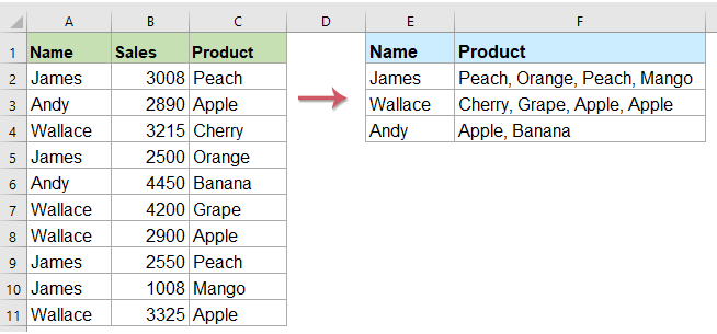
Fel rheol, yn Excel, pan fyddwch chi'n defnyddio'r swyddogaeth VLOOKUP, os oes sawl gwerth i gyd-fynd â'r meini prawf, gallwch chi gael yr un cyntaf. Ond, weithiau, rydych chi am ddychwelyd yr holl werthoedd cyfatebol sy'n cwrdd â'r meini prawf i mewn i un gell fel y dangosir y screenshot canlynol, sut allech chi ei ddatrys?
- Vlookup i ddychwelyd yr holl werthoedd paru yn un gell
- Vlookup i ddychwelyd yr holl werthoedd paru heb ddyblygu i mewn i un gell
Vlookup i ddychwelyd gwerthoedd lluosog i mewn i un gell gyda Swyddogaeth Diffiniedig Defnyddiwr
- Vlookup i ddychwelyd yr holl werthoedd paru yn un gell
- Vlookup i ddychwelyd yr holl werthoedd paru heb ddyblygu i mewn i un gell
Vlookup i ddychwelyd gwerthoedd lluosog i mewn i un gell gyda nodwedd ddefnyddiol
Vlookup i ddychwelyd gwerthoedd lluosog i mewn i un gell â swyddogaeth TEXTJOIN (Excel 2019 ac Office 365)
Os oes gennych y fersiwn uwch o'r Excel fel Excel 2019 ac Office 365, mae swyddogaeth newydd - TEXTJOIN, gyda'r swyddogaeth bwerus hon, gallwch chi edrych yn gyflym a dychwelyd yr holl werthoedd paru i mewn i un cell.
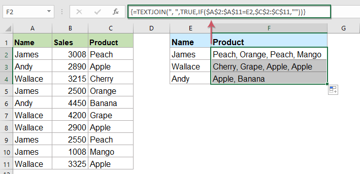
Vlookup i ddychwelyd yr holl werthoedd paru yn un gell
Defnyddiwch y fformiwla isod mewn cell wag lle rydych chi am roi'r canlyniad, yna pwyswch Ctrl + Shift + Enter allweddi gyda'i gilydd i gael y canlyniad cyntaf, ac yna llusgwch y ddolen llenwi i lawr i'r gell rydych chi am ddefnyddio'r fformiwla hon, a byddwch chi'n cael yr holl werthoedd cyfatebol fel y dangosir isod y screenshot:
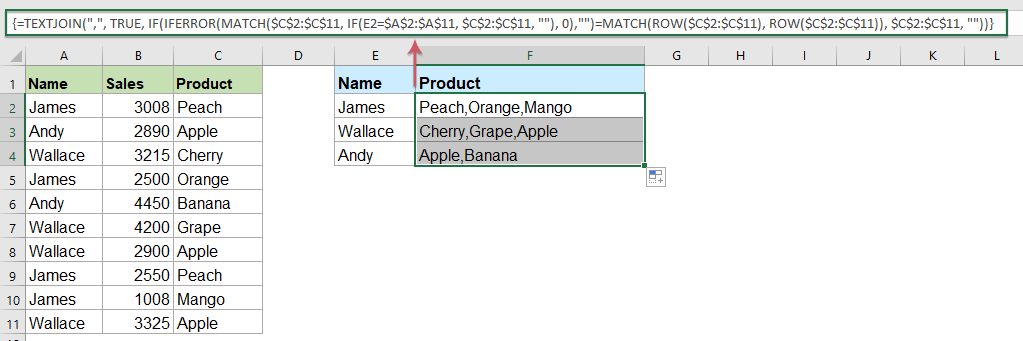
Vlookup i ddychwelyd yr holl werthoedd paru heb ddyblygu i mewn i un gell
Os ydych chi am ddychwelyd yr holl werthoedd paru yn seiliedig ar y data edrych heb ddyblygu, gall y fformiwla isod eich helpu chi.
Copïwch a gludwch y fformiwla ganlynol i mewn i gell wag, yna pwyswch Ctrl + Shift + Enter allweddi gyda'i gilydd i gael y canlyniad cyntaf, ac yna copïwch y fformiwla hon i lenwi celloedd eraill, a byddwch yn cael yr holl werthoedd cyfatebol heb y rhai dulpicate fel y dangosir isod y screenshot:
Vlookup i ddychwelyd gwerthoedd lluosog i mewn i un gell gyda Swyddogaeth Diffiniedig Defnyddiwr
Dim ond ar gyfer Excel 2019 ac Office 365 y mae'r swyddogaeth TEXTJOIN uchod ar gael, os oes gennych fersiynau Excel is eraill, dylech ddefnyddio rhai codau ar gyfer gorffen y dasg hon.
Vlookup i ddychwelyd yr holl werthoedd paru yn un gell
1. Daliwch i lawr y ALT + F11 allweddi, ac mae'n agor y Microsoft Visual Basic ar gyfer Ceisiadau ffenestr.
2. Cliciwch Mewnosod > Modiwlau, a gludwch y cod canlynol yn y Ffenestr Modiwl.
Cod VBA: Vlookup i ddychwelyd gwerthoedd lluosog i mewn i un gell
Function ConcatenateIf(CriteriaRange As Range, Condition As Variant, ConcatenateRange As Range, Optional Separator As String = ",") As Variant
'Updateby Extendoffice
Dim xResult As String
On Error Resume Next
If CriteriaRange.Count <> ConcatenateRange.Count Then
    ConcatenateIf = CVErr(xlErrRef)
    Exit Function
End If
For i = 1 To CriteriaRange.Count
    If CriteriaRange.Cells(i).Value = Condition Then
        xResult = xResult & Separator & ConcatenateRange.Cells(i).Value
    End If
Next i
If xResult <> "" Then
    xResult = VBA.Mid(xResult, VBA.Len(Separator) + 1)
End If
ConcatenateIf = xResult
Exit Function
End Function
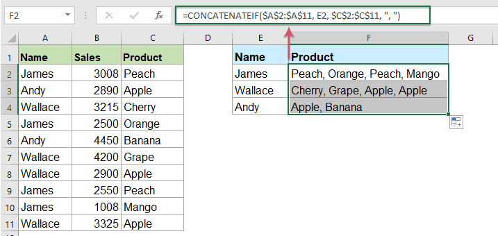
3. Yna arbedwch a chau'r cod hwn, ewch yn ôl i'r daflen waith, a nodi'r fformiwla hon: =CONCATENATEIF($A$2:$A$11, E2, $C$2:$C$11, ", ") i mewn i gell wag benodol lle rydych chi am osod y canlyniad, yna llusgwch y ddolen llenwi i lawr i gael yr holl werthoedd cyfatebol mewn un cell rydych chi ei eisiau, gweler y screenshot:
Vlookup i ddychwelyd yr holl werthoedd paru heb ddyblygu i mewn i un gell
Er mwyn anwybyddu'r dyblygu yn y gwerthoedd paru a ddychwelwyd, gwnewch y cod isod.
1. Daliwch i lawr y Alt + F11 allweddi i agor y Microsoft Visual Basic ar gyfer Ceisiadau ffenestr.
2. Cliciwch Mewnosod > Modiwlau, a gludwch y cod canlynol yn y Ffenestr Modiwl.
Cod VBA: Vlookup a dychwelyd nifer o werthoedd cyfatebol unigryw i mewn i un gell
Function MultipleLookupNoRept(Lookupvalue As String, LookupRange As Range, ColumnNumber As Integer)
'Updateby Extendoffice
    Dim xDic As New Dictionary
    Dim xRows As Long
    Dim xStr As String
    Dim i As Long
    On Error Resume Next
    xRows = LookupRange.Rows.Count
    For i = 1 To xRows
        If LookupRange.Columns(1).Cells(i).Value = Lookupvalue Then
            xDic.Add LookupRange.Columns(ColumnNumber).Cells(i).Value, ""
        End If
    Next
    xStr = ""
    MultipleLookupNoRept = xStr
    If xDic.Count > 0 Then
        For i = 0 To xDic.Count - 1
            xStr = xStr & xDic.Keys(i) & ","
        Next
        MultipleLookupNoRept = Left(xStr, Len(xStr) - 1)
    End If
End Function
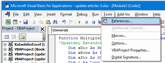
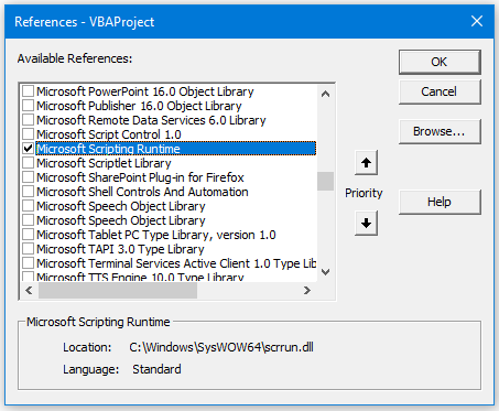
3. Ar ôl mewnosod y cod, yna cliciwch offer > Cyfeiriadau yn yr agored Microsoft Visual Basic ar gyfer Ceisiadau ffenestr, ac yna, yn y popped allan Cyfeiriadau - VBAProject blwch deialog, gwirio Amser Rhedeg Sgriptio Microsoft opsiwn yn y Cyfeiriadau sydd ar Gael blwch rhestr, gweler sgrinluniau:
 |
 |
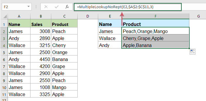
4. Yna cliciwch OK i gau'r blwch deialog, cadw a chau'r ffenestr god, dychwelyd i'r daflen waith, a nodi'r fformiwla hon: =MultipleLookupNoRept(E2,$A$2:$C$11,3) into a blank cell where you want to output the result, and then drag the fill hanlde down to get all matching values, see screenshot:
Vlookup i ddychwelyd gwerthoedd lluosog i mewn i un gell gyda nodwedd ddefnyddiol
Os oes gennych ein Kutools ar gyfer Excel, Gyda'i Rhesi Cyfuno Uwch nodwedd, gallwch chi uno neu gyfuno'r rhesi yn gyflym yn seiliedig ar yr un gwerth a gwneud rhai cyfrifiadau ag sydd eu hangen arnoch chi.
Ar ôl gosod Kutools ar gyfer Excel, gwnewch fel a ganlyn:
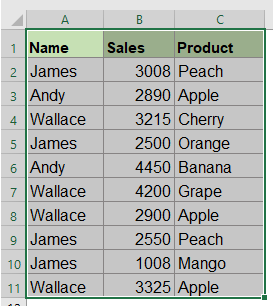
1. Dewiswch yr ystod ddata rydych chi am gyfuno data un golofn yn seiliedig ar golofn arall.
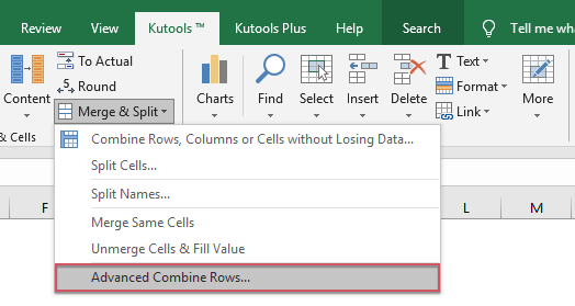
2. Cliciwch Kutools > Uno a Hollti > Rhesi Cyfuno Uwch, gweler y screenshot:
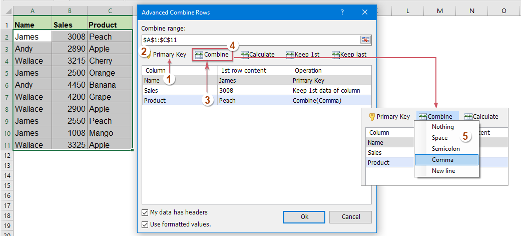
3. Yn y popped allan Rhesi Cyfuno Uwch blwch deialog:
- Cliciwch enw'r golofn allweddol i'w chyfuno yn seiliedig ar, ac yna cliciwch Allwedd Cynradd
- Yna cliciwch colofn arall yr ydych am gyfuno ei data yn seiliedig ar y golofn allweddol, a chlicio Cyfunwch i ddewis un gwahanydd ar gyfer gwahanu'r data cyfun.
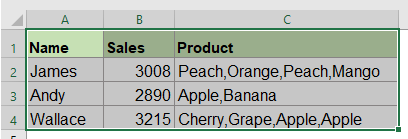
4. Yna cliciwch OK botwm, a byddwch yn cael y canlyniadau canlynol:
 |
 |
Dadlwythwch a threial am ddim Kutools ar gyfer Excel Nawr !
Erthyglau mwy cymharol:
- Swyddogaeth VLOOKUP Gyda Rhai Enghreifftiau Sylfaenol ac Uwch
- Yn Excel, mae swyddogaeth VLOOKUP yn swyddogaeth bwerus i'r rhan fwyaf o ddefnyddwyr Excel, a ddefnyddir i chwilio am werth yn y chwith mwyaf o'r ystod ddata, a dychwelyd gwerth paru yn yr un rhes o golofn a nodwyd gennych. Mae'r tiwtorial hwn yn siarad am sut i ddefnyddio swyddogaeth VLOOKUP gyda rhai enghreifftiau sylfaenol ac uwch yn Excel.
- Dychwelwch werthoedd paru lluosog yn seiliedig ar un neu fwy o feini prawf
- Fel rheol, mae'n hawdd i'r mwyafrif ohonom edrych ar werth penodol a dychwelyd yr eitem baru trwy ddefnyddio'r swyddogaeth VLOOKUP. Ond, a ydych erioed wedi ceisio dychwelyd gwerthoedd paru lluosog yn seiliedig ar un neu fwy o feini prawf? Yn yr erthygl hon, byddaf yn cyflwyno rhai fformiwlâu ar gyfer datrys y dasg gymhleth hon yn Excel.
- Vlookup A Dychwelyd Gwerthoedd Lluosog yn Fertigol
- Fel rheol, gallwch ddefnyddio'r swyddogaeth Vlookup i gael y gwerth cyfatebol cyntaf, ond, weithiau, rydych chi am ddychwelyd yr holl gofnodion paru yn seiliedig ar faen prawf penodol. Yr erthygl hon, byddaf yn siarad am sut i wylio a dychwelyd yr holl werthoedd paru yn fertigol, yn llorweddol neu i mewn i un gell.
- Vlookup A Dychwelyd Gwerthoedd Lluosog O'r Rhestr Gostwng
- Yn Excel, sut allech chi wylio a dychwelyd sawl gwerth cyfatebol o gwymplen, sy'n golygu pan fyddwch chi'n dewis un eitem o'r gwymplen, mae ei holl werthoedd cymharol yn cael eu harddangos ar unwaith. Yr erthygl hon, byddaf yn cyflwyno'r datrysiad gam wrth gam.
Offer Cynhyrchiant Swyddfa Gorau
Supercharge Eich Sgiliau Excel gyda Kutools ar gyfer Excel, a Phrofiad Effeithlonrwydd Fel Erioed Erioed. Kutools ar gyfer Excel Yn Cynnig Dros 300 o Nodweddion Uwch i Hybu Cynhyrchiant ac Arbed Amser. Cliciwch Yma i Gael Y Nodwedd Sydd Ei Angen Y Mwyaf...
")
Mae Office Tab yn dod â rhyngwyneb Tabbed i Office, ac yn Gwneud Eich Gwaith yn Haws o lawer
- Galluogi golygu a darllen tabbed yn Word, Excel, PowerPoint, Cyhoeddwr, Mynediad, Visio a Phrosiect.
- Agor a chreu dogfennau lluosog mewn tabiau newydd o'r un ffenestr, yn hytrach nag mewn ffenestri newydd.
- Yn cynyddu eich cynhyrchiant 50%, ac yn lleihau cannoedd o gliciau llygoden i chi bob dydd!
")