Skip i'r prif gynnwys

Sut i gyd-fynd â chelloedd os yw'r un gwerth yn bodoli mewn colofn arall yn Excel?

Fel y dangosir yn y sgrin isod, os ydych chi am gydgatenu celloedd yn yr ail golofn yn seiliedig ar yr un gwerthoedd yn y golofn gyntaf, mae yna nifer o ddulliau y gallwch eu defnyddio. Yn yr erthygl hon, byddwn yn cyflwyno tair ffordd o gyflawni'r dasg hon.

cyfuno os yr un peth


Concatenate celloedd os yw'r un gwerth â fformwlâu a hidlydd

Mae'r fformiwlâu canlynol yn helpu i gydgatenu cynnwys y celloedd cyfatebol mewn colofn yn seiliedig ar yr un gwerth mewn colofn arall.

1. Dewiswch gell wag ar wahân i'r ail golofn (yma rydyn ni'n dewis cell C2), nodwch y fformiwla = OS (A2 <> A1, B2, C1 & "," & B2) i mewn i'r bar fformiwla, ac yna pwyswch y Rhowch allweddol.

2. Yna dewiswch gell C2, a llusgwch y Llenwi Trin i lawr i gelloedd y mae angen i chi eu cyd-daro.

3. Rhowch fformiwla = OS (A2 <> A3, CONCATENATE (A2, "," "", C2, "" ""), "") i mewn i gell D2, a llusgo Llenwch Trin i lawr i'r celloedd gorffwys.

4. Dewiswch gell D1, a chlicio Dyddiad > Hidlo. Gweler y screenshot:

5. Cliciwch y gwymplen yng nghell D1, dad-diciwch y (Bylchau) blwch, ac yna cliciwch ar y OK botwm.

Gallwch weld bod y celloedd yn cyd-daro os yw gwerthoedd y golofn gyntaf yr un peth.

Nodyn: Er mwyn defnyddio'r fformwlâu uchod yn llwyddiannus, rhaid i'r un gwerthoedd yng ngholofn A fod yn barhaus.


Cydgatenate celloedd yn hawdd os yw'r un gwerth â Kutools ar gyfer Excel (sawl clic)

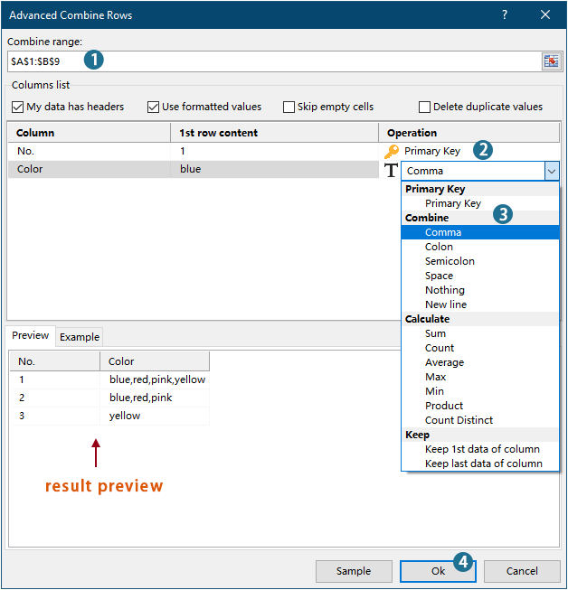
Mae'r dull a ddisgrifir uchod yn gofyn am greu dwy golofn cynorthwyydd ac mae'n cynnwys sawl cam, a all fod yn anghyfleus. Os ydych chi'n chwilio am ffordd symlach, ystyriwch ddefnyddio'r Rhesi Cyfuno Uwch offeryn o Kutools ar gyfer Excel. Gyda dim ond ychydig o gliciau, mae'r cyfleustodau hwn yn caniatáu ichi gydgatenu celloedd gan ddefnyddio amffinydd penodol, gan wneud y broses yn gyflym ac yn ddi-drafferth.

Tip: Cyn gwneud cais offeryn hwn, os gwelwch yn dda gosod Kutools ar gyfer Excel yn gyntaf. Ewch i lawrlwytho am ddim nawr.

1. Cliciwch Kutools > Uno a Hollti > Rhesi Cyfuno Uwch i alluogi'r nodwedd hon.
2. Yn y Rhesi Cyfuno Uwch blwch deialog, does ond angen i chi:
  • Dewiswch yr ystod rydych chi am ei chydgatenu;
  • Gosodwch y golofn gyda'r un gwerthoedd â'r Allwedd Cynradd colofn.
  • Nodwch wahanydd i gyfuno'r celloedd.
  • Cliciwch OK.

Canlyniad

Nodyn:

Concatenate celloedd os yw'r un gwerth â chod VBA

Gallwch hefyd ddefnyddio cod VBA i gydgatenu celloedd mewn colofn os yw'r un gwerth yn bodoli mewn colofn arall.

1. Gwasgwch Alt + F11 allweddi i agor y Cymwysiadau Sylfaenol Gweledol Microsoft ffenestr.

2. Yn y Cymwysiadau Sylfaenol Gweledol Microsoft ffenestr, cliciwch Mewnosod > Modiwlau. Yna copïwch a gludwch y cod isod i'r Modiwlau ffenestr.

Cod VBA: cyd-fynd â chelloedd os yw'r un gwerthoedd

Sub ConcatenateCellsIfSameValues()
	Dim xCol As New Collection
	Dim xSrc As Variant
	Dim xRes() As Variant
	Dim I As Long
	Dim J As Long
	Dim xRg As Range
	xSrc    = Range("A1", Cells(Rows.Count, "A").End(xlUp)).Resize(, 2)
	Set xRg = Range("D1")
	On Error Resume Next
	For I = 2 To UBound(xSrc)
		xCol.Add xSrc(I, 1), TypeName(xSrc(I, 1)) & CStr(xSrc(I, 1))
	Next I
	On Error GoTo 0
	ReDim xRes(1 To xCol.Count + 1, 1 To 2)
	xRes(1, 1) = "No"
	xRes(1, 2) = "Combined Color"
	For I = 1 To xCol.Count
		xRes(I + 1, 1) = xCol(I)
		For J = 2 To UBound(xSrc)
			If xSrc(J, 1) = xRes(I + 1, 1) Then
				xRes(I + 1, 2) = xRes(I + 1, 2) & ", " & xSrc(J, 2)
			End If
		Next J
		xRes(I + 1, 2) = Mid(xRes(I + 1, 2), 2)
	Next I
	Set xRg = xRg.Resize(UBound(xRes, 1), UBound(xRes, 2))
	xRg.NumberFormat = "@"
	xRg = xRes
	xRg.EntireColumn.AutoFit
End Sub

Nodiadau:

1. D1 yn y llinell Gosod xRg = Ystod ("D1") yn golygu y bydd y canlyniad yn cael ei osod gan ddechrau gyda cell D1.
2. "Na"ac "Lliw Cyfunol" yn y llinell xRes (1, 1) = "Na" a xRes (1, 2) = "Lliw Cyfun" yw penawdau colofnau dethol. 

3. Gwasgwch y F5 allwedd i redeg y cod, yna byddwch yn cael y canlyniadau cydgysylltiedig mewn ystod benodol.


Cydgatenate celloedd yn hawdd os yw'r un gwerth â Kutools ar gyfer Excel

Offer Cynhyrchiant Swyddfa Gorau

🤖 Kutools AI Aide: Chwyldro dadansoddi data yn seiliedig ar: Cyflawniad Deallus   |  Cynhyrchu Cod  |  Creu Fformiwlâu Personol  |  Dadansoddi Data a Chynhyrchu Siartiau  |  Invoke Swyddogaethau Kutools...
Nodweddion Poblogaidd: Darganfod, Amlygu neu Adnabod Dyblygiadau   |  Dileu Rhesi Gwag   |  Cyfuno Colofnau neu Gelloedd heb Colli Data   |   Rownd heb Fformiwla ...
Super-edrych: VLookup Meini Prawf Lluosog    VLookup Gwerth Lluosog  |   VLookup Ar Draws Taflenni Lluosog   |   Edrych Niwlog ....
Rhestr gwympo Uwch: Creu Rhestr Gollwng yn Gyflym   |  Rhestr Gollwng Dibynnol   |  Rhestr Gollwng Aml-ddewis ....
Rheolwr Colofn: Ychwanegu Nifer Penodol o Golofnau  |  Symud Colofnau  |  Toglo Statws Gwelededd Colofnau Cudd  |  Cymharwch Ystodau a Cholofnau ...
Nodweddion dan Sylw: Ffocws ar y Grid   |  Golwg Dylunio   |   Bar Fformiwla Mawr    Rheolwr Llyfr Gwaith a Thaflen   |  Llyfrgell Adnoddau (Testun Auto)   |  Dewiswr Dyddiad   |  Cyfuno Taflenni Gwaith   |  Amgryptio/Dadgryptio Celloedd    Anfon E-byst trwy Restr   |  Hidlo Super   |   Hidlo Arbennig (hidlo mewn print trwm/italig/strikethrough...) ...
15 Set Offer Gorau12 Testun offer (Ychwanegu Testun, Dileu Cymeriadau,...)   |   50 + Siart Mathau (Siart Gantt,...)   |   40+ Ymarferol Fformiwlâu (Cyfrifwch oedran yn seiliedig ar ben-blwydd,...)   |   19 mewnosod offer (Mewnosod Cod QR, Mewnosod Llun o'r Llwybr,...)   |   12 Trosi offer (Rhifau i Eiriau, Trosi arian cyfred,...)   |   7 Uno a Hollti offer (Rhesi Cyfuno Uwch, Celloedd Hollt,...)   |   ... a mwy

Supercharge Eich Sgiliau Excel gyda Kutools ar gyfer Excel, a Phrofiad Effeithlonrwydd Fel Erioed Erioed. Kutools ar gyfer Excel Yn Cynnig Dros 300 o Nodweddion Uwch i Hybu Cynhyrchiant ac Arbed Amser.  Cliciwch Yma i Gael Y Nodwedd Sydd Ei Angen Y Mwyaf...

Disgrifiad


Mae Office Tab yn dod â rhyngwyneb Tabbed i Office, ac yn Gwneud Eich Gwaith yn Haws o lawer

  • Galluogi golygu a darllen tabbed yn Word, Excel, PowerPoint, Cyhoeddwr, Mynediad, Visio a Phrosiect.
  • Agor a chreu dogfennau lluosog mewn tabiau newydd o'r un ffenestr, yn hytrach nag mewn ffenestri newydd.
  • Yn cynyddu eich cynhyrchiant 50%, ac yn lleihau cannoedd o gliciau llygoden i chi bob dydd!
Comments (23)
No ratings yet. Be the first to rate!
This comment was minimized by the moderator on the site
thank you very much, the VBA code works very well but I have a question that I can't solve.

NO Color
1 red
1 blue
1 red
1 yellow
2 red
2 yellow


in this case, in column B we have some duplicate colors related to the same number. How can I have an output that only return the values once?

I would like an output like this

NO Color
1 red, blue, yellow
2 red, yellow
This comment was minimized by the moderator on the site
Hi

The second method described in the post can help you solve this problem. After following the steps to specify the settings, checking the Delect Duplicate Values option will delete all duplicates in the combined results.
https://www.extendoffice.com/images/stories/comments/comment-picture-zxm/concatenate.png
This comment was minimized by the moderator on the site
Thank you so much for this formula! It saved hours of investigation! Fantastic work :)
This comment was minimized by the moderator on the site
Hi Crystal,

Thanks for your reply. I'll have to put my thinking hat on again...
Thank you
This comment was minimized by the moderator on the site
Hello, the macro above works great! Thank you. Is it anyway possible (I tried, but not successful) to amend it to concatenate column B (description) based on duplicates in column A (HS code) but also taking column C (origin) in the combination?
So description texts concatenate per HS code per origin.
Also column D(quantity) and column E(value) must be summed per HS code and origin.

A B C D E
HS CODE DESCRIPTION ORIGIN QUANTITY VALUE
5407420000 TWEED CN 10 € 150,00
5407420000 COTTON CN 15 € 250,00
5407420000 POLYESTER TW 5 € 130,00
5407420000 ORGANIC COTTON US 18 € 450,00
5407420000 COTTON US 23 € 780,00
5407420000 VELVET DELUXE CN 20 € 380,00
5407420000 COTTON CN 10 € 120,00
5806310000 TWEED JP 15 € 35,00
5806310000 POLYESTER AU 20 € 78,00
5806310000 TWEED AU 25 € 254,00
5806310000 POLYESTER SG 130 € 888,00
5806310000 COTTON EU 120 € 945,00
5806310000 COTTON FABRIC EU 10 € 80,00


Result shopuld be:

5407420000 TWEED, COTTON, VELVET DULUXE, COTTON, CN 55 € 900,00
5407420000 POLYESTER TW 5 € 130,00
5407420000 ORGANIC COTTON, COTTON US 41 € 1230,00
5806310000 TWEED JP 15 € 35,00
5806310000 POLYESTER, TWEED AU 45 € 332,00
5806310000 POLYESTER SG 130 € 888,00
5806310000 COTTON, COTTON FABRIC EU 130 € 1025,00

I hope this possible, thank you!
This comment was minimized by the moderator on the site
Hi Ivar,

Thank you for your comment. I am not able to solve this problem with VBA code yet. Sorry for that.
You can try if the last method can help.
This comment was minimized by the moderator on the site
Hello, how would the VBA code be adjusted if I want to combine cells in column M based on the duplicates in column A?
This comment was minimized by the moderator on the site
Hi Kristin,To combine cells in column M based on the duplicates in column A, try the VBA below.In the code,  O1 is the first cell to output the results; M is the column you will combine based on the duplicates in column A; A1 and A represent the first cell and the column where the duplicates locate; No and Combine color is the header of the columns after concatenating. You can change these variables as needed.<div data-tag="code">Sub ConcatenateCellsIfSameValues()
'Updated by Extendoffice 20211105
Dim xCol As New Collection
Dim xSrc As Variant
Dim xSrcValue As Variant
Dim xRes() As Variant
Dim I As Long
Dim J As Long
Dim xRg As Range
Dim xResultAddress As String
Dim xMergeAddress As String
Dim xUp As Integer

xResultAddress = "O1" 'The cell to output the results
xMergeAddress = "M" 'The column you will combine based on the duplicates in column A

xSrc = Range("A1", Cells(Rows.Count, "A").End(xlUp)).Resize(, 1)
xUp = Range("A1", Cells(Rows.Count, "A").End(xlUp)).Rows.Count
xSrcValue = Range(xMergeAddress & "1:" & xMergeAddress & xUp)

Set xRg = Range(xResultAddress)
On Error Resume Next
For I = 2 To UBound(xSrc)
xCol.Add xSrc(I, 1), TypeName(xSrc(I, 1)) & CStr(xSrc(I, 1))
Next I

On Error GoTo 0
ReDim xRes(1 To xCol.Count + 1, 1 To 2)
xRes(1, 1) = "No"
xRes(1, 2) = "Combined Color"
For I = 1 To xCol.Count
xRes(I + 1, 1) = xCol(I)
For J = 2 To UBound(xSrc)
If xSrc(J, 1) = xRes(I + 1, 1) Then
xRes(I + 1, 2) = xRes(I + 1, 2) & ", " & xSrcValue(J, 1)
End If
Next J
xRes(I + 1, 2) = Mid(xRes(I + 1, 2), 2)
Next I
Set xRg = xRg.Resize(UBound(xRes, 1), UBound(xRes, 2))
xRg.NumberFormat = "@"
xRg = xRes
xRg.EntireColumn.AutoFit
End Sub
This comment was minimized by the moderator on the site
I just wanted to thank you. It wasn't exactly what I wanted but man did it help me figure out what to do.

I have a table where the person's name was in column A, dates in column B and the names of tools they use in the headers of columns C:G . In each column there is a "Y" if they used that tool on that date and blank if they did not. (FYI: the same person can be listed more than once and may have used the same tool more than once) On a separate (summary) page I wanted to list all tools each person used within a date period, only listing each tool they used once, in the same cell. On this page, the person's name was in column A, Types of tools used in column B and the helper columns were in column G:K. Here's what I got:
The first helper column (G2):
=IF(COUNTIFS(Table7[Person's Name],A2,Table7[Screw Driver],"Y",Table7[Date],">="&1/1/20,Table7[Date],"<="&3/31/20),"Screw Driver","")
In the last helper column (K2):
=IF(COUNTIFS(Table7[Person's Name],A2,Table7[Hammer],"Y",Table7[Date],">="&1/1/20,Table7[Date],"<="&3/31/20),IF(J2="","Hammer",J2&"/"&"Hammer"),J2)

In B2 I just entered =K2

Thanks again and I hope this helps someone. EZPD
This comment was minimized by the moderator on the site
Hi, first of all thanks for creating this resource. I have been trying to figure this out for a couple of hours and I'm stuck. I'm using your 'concatenate cells if same value' but my script is looking at column "D" instead of "A. I can't figure out how to get it to use a different column for the data besides the one right next to it. In my cases I want it to look at column "D" to see if the value is the same and if so, it will grab the data from column "H" and put that data from column "H' into a cell in column "J". How do I switch this to use column "H" for the data? Thx


Sub ConcatenateCellsIfSameValues()
Dim xCol As New Collection
Dim xSrc As Variant
Dim xRes() As Variant
Dim I As Long
Dim J As Long
Dim xRg As Range
xSrc = Range("D1", Cells(Rows.Count, "D").End(xlUp)).Resize(, 2)
Set xRg = Range("J1")
On Error Resume Next
For I = 2 To UBound(xSrc)
xCol.Add xSrc(I, 1), TypeName(xSrc(I, 1)) & CStr(xSrc(I, 1))
Next I
On Error GoTo 0
ReDim xRes(1 To xCol.Count + 1, 1 To 2)
xRes(1, 1) = "No"
xRes(1, 2) = "Products"
For I = 1 To xCol.Count
xRes(I + 1, 1) = xCol(I)
For J = 2 To UBound(xSrc)
If xSrc(J, 1) = xRes(I + 1, 1) Then
xRes(I + 1, 2) = xRes(I + 1, 2) & vbCrLf & xSrc(J, 2)
End If
Next J
xRes(I + 1, 2) = Mid(xRes(I + 1, 2), 2)
Next I
Set xRg = xRg.Resize(UBound(xRes, 1), UBound(xRes, 2))
xRg.NumberFormat = "@"
xRg = xRes
xRg.EntireColumn.AutoFit
End Sub
This comment was minimized by the moderator on the site
"I can't figure out how to get it to use a different column for the data besides the one right next to it. In my cases I want it to look at column 'D' to see if the value is the same and if so, it will grab the data from column 'H' and put that data from column 'H' into a cell in column 'J'."

Did you ever figure this out?
This comment was minimized by the moderator on the site
Hi,

looks like 2 of your formulas are wrong :

=IF(A2<>A3,CONCATENATE(A2,",""",C2,""""),""). You need to change "A2" to "D1". As you'll want to add the string to the previous cell.

same goes for this formula :

=IF(A2<>A1,B2,C1 & "," & B2) : Change C1 to D1.


kind regards


Harry
This comment was minimized by the moderator on the site
I use this VBA for lots of my spreadsheets and its great. But the spreadsheets have become very large 50k+ rows and it doesnt seem to be working any more. If I use it on 1000 rows it works fine but large sets of data it cant seem to cope with. No errors just no results. Any help would be appreciated.
This comment was minimized by the moderator on the site
Hi James,
I tested the code as you mentioned, but it still works well in my case even I set the rows to 1000+.
This comment was minimized by the moderator on the site
Using the VBA macro and getting great results, I have tried tweaking it slightly for my needs but cant get it to work so I hope you can help.

Which bit do I change to make it concat a specific column, not the one directly to the right of the xSrc = Range?

Thanks for your great work!
This comment was minimized by the moderator on the site
Or as a better option, if you had 3 columns instead of 2 and found duplicates in column A (like your example) can you concat column B into a cell and column C into a seperate cell? So if you had columns of Number, Colour, Age, could you concat colour and age into different columns upon finding duplicates in Number? Hope that makes sense!
There are no comments posted here yet
Load More
Please leave your comments in English
Posting as Guest
×
Rate this post:
0   Characters
Suggested Locations