Skip i'r prif gynnwys

Sut i dynnu sylw at y gwerth agosaf mewn rhestr at rif penodol yn Excel?

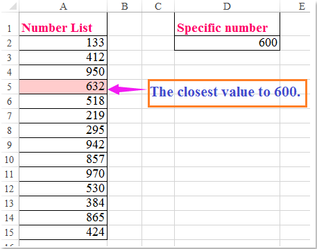
Gan dybio, mae gennych chi restr o rifau, nawr, efallai yr hoffech chi dynnu sylw at y gwerthoedd agosaf neu sawl gwerth agosaf yn seiliedig ar rif penodol fel y screenshot canlynol a ddangosir. Yma, efallai y bydd yr erthygl hon yn eich helpu i ddatrys y dasg hon yn rhwydd.

doc tynnu sylw at y gwerth agosaf 1
doc tynnu sylw at y gwerth agosaf 2

Tynnwch sylw at y gwerthoedd n agosaf neu agosaf at rif penodol gyda Fformatio Amodol


swigen dde glas saeth Tynnwch sylw at y gwerthoedd n agosaf neu agosaf at rif penodol gyda Fformatio Amodol

I dynnu sylw at y gwerth agosaf yn seiliedig ar y rhif penodol, gwnewch fel a ganlyn:

1. Dewiswch y rhestr rifau rydych chi am dynnu sylw ati, ac yna cliciwch Hafan > Fformatio Amodol > Rheol Newydd, gweler y screenshot:

doc tynnu sylw at y gwerth agosaf 3

2. Yn y Rheol Fformatio Newydd blwch deialog, gwnewch y gweithrediadau canlynol:

(1.) Cliciwch Defnyddiwch fformiwla i bennu pa gelloedd i'w fformatio O dan y Dewiswch Math o Reol blwch rhestr;

(2.) Yn y Gwerthoedd fformat lle mae'r fformiwla hon yn wir blwch testun, nodwch y fformiwla hon: =ABS(A2-$D$2)=MIN(ABS($A$2:$A$15-$D$2)) (A2 yw'r gell gyntaf yn eich rhestr ddata, D2 yw'r rhif penodol y byddwch chi'n ei gymharu, A2: A15 yw'r rhestr rifau rydych chi am dynnu sylw at y gwerth agosaf ohoni.)

doc tynnu sylw at y gwerth agosaf 4

3. Yna cliciwch fformat botwm i fynd y Celloedd Fformat blwch deialog, o dan y Llenwch tab, dewiswch un lliw yr ydych chi'n ei hoffi, gweler y screenshot:

doc tynnu sylw at y gwerth agosaf 5

4. Ac yna cliciwch OK > OK i gau'r deialogau, amlygwyd y gwerth agosaf at y rhif penodol ar unwaith, gweler y screenshot:

doc tynnu sylw at y gwerth agosaf 6

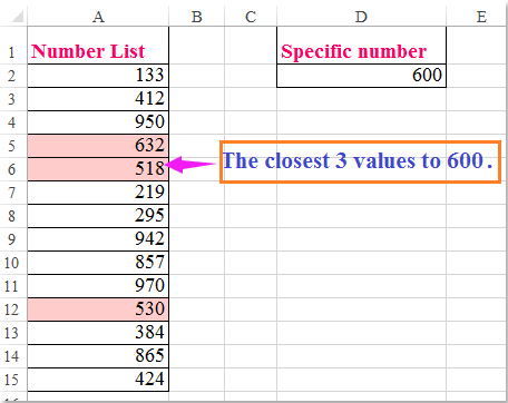
Awgrymiadau: Os ydych chi am dynnu sylw at y 3 gwerth agosaf at y gwerthoedd a roddir, gallwch gymhwyso'r fformiwla hon yn y Fformatio Amodol, =ISNUMBER(MATCH(ABS($D$2-A2),SMALL(ABS($D$2-$A$2:$A$15),ROW($1:$3)),0)), gweler y screenshot:

doc tynnu sylw at y gwerth agosaf 7

Nodyn: Yn y fformiwla uchod: A2 yw'r gell gyntaf yn eich rhestr ddata, D2 yw'r rhif penodol y byddwch chi'n ei gymharu, A2: A15 yw'r rhestr rifau rydych chi am dynnu sylw at y gwerth agosaf ohoni, $ 1: $ 3 yn nodi y bydd y tri gwerth agosaf yn cael eu hamlygu. Gallwch eu newid i'ch angen.

Offer Cynhyrchiant Swyddfa Gorau

🤖 Kutools AI Aide: Chwyldro dadansoddi data yn seiliedig ar: Cyflawniad Deallus   |  Cynhyrchu Cod  |  Creu Fformiwlâu Personol  |  Dadansoddi Data a Chynhyrchu Siartiau  |  Invoke Swyddogaethau Kutools...
Nodweddion Poblogaidd: Darganfod, Amlygu neu Adnabod Dyblygiadau   |  Dileu Rhesi Gwag   |  Cyfuno Colofnau neu Gelloedd heb Colli Data   |   Rownd heb Fformiwla ...
Super-edrych: VLookup Meini Prawf Lluosog    VLookup Gwerth Lluosog  |   VLookup Ar Draws Taflenni Lluosog   |   Edrych Niwlog ....
Rhestr gwympo Uwch: Creu Rhestr Gollwng yn Gyflym   |  Rhestr Gollwng Dibynnol   |  Rhestr Gollwng Aml-ddewis ....
Rheolwr Colofn: Ychwanegu Nifer Penodol o Golofnau  |  Symud Colofnau  |  Toglo Statws Gwelededd Colofnau Cudd  |  Cymharwch Ystodau a Cholofnau ...
Nodweddion dan Sylw: Ffocws ar y Grid   |  Golwg Dylunio   |   Bar Fformiwla Mawr    Rheolwr Llyfr Gwaith a Thaflen   |  Llyfrgell Adnoddau (Testun Auto)   |  Dewiswr Dyddiad   |  Cyfuno Taflenni Gwaith   |  Amgryptio/Dadgryptio Celloedd    Anfon E-byst trwy Restr   |  Hidlo Super   |   Hidlo Arbennig (hidlo mewn print trwm/italig/strikethrough...) ...
15 Set Offer Gorau12 Testun offer (Ychwanegu Testun, Dileu Cymeriadau,...)   |   50 + Siart Mathau (Siart Gantt,...)   |   40+ Ymarferol Fformiwlâu (Cyfrifwch oedran yn seiliedig ar ben-blwydd,...)   |   19 mewnosod offer (Mewnosod Cod QR, Mewnosod Llun o'r Llwybr,...)   |   12 Trosi offer (Rhifau i Eiriau, Trosi arian cyfred,...)   |   7 Uno a Hollti offer (Rhesi Cyfuno Uwch, Celloedd Hollt,...)   |   ... a mwy

Supercharge Eich Sgiliau Excel gyda Kutools ar gyfer Excel, a Phrofiad Effeithlonrwydd Fel Erioed Erioed. Kutools ar gyfer Excel Yn Cynnig Dros 300 o Nodweddion Uwch i Hybu Cynhyrchiant ac Arbed Amser.  Cliciwch Yma i Gael Y Nodwedd Sydd Ei Angen Y Mwyaf...

Disgrifiad


Mae Office Tab yn dod â rhyngwyneb Tabbed i Office, ac yn Gwneud Eich Gwaith yn Haws o lawer

  • Galluogi golygu a darllen tabbed yn Word, Excel, PowerPoint, Cyhoeddwr, Mynediad, Visio a Phrosiect.
  • Agor a chreu dogfennau lluosog mewn tabiau newydd o'r un ffenestr, yn hytrach nag mewn ffenestri newydd.
  • Yn cynyddu eich cynhyrchiant 50%, ac yn lleihau cannoedd o gliciau llygoden i chi bob dydd!
Comments (8)
No ratings yet. Be the first to rate!
This comment was minimized by the moderator on the site
=ABS(A2-$D$2)=MIN(ABS($A$2:$A$15-$D$2)) данная формула не работает. Пробовал exel 2010 и 2013. Если использовать вторую формулу, ругается на ошибку.
This comment was minimized by the moderator on the site
Hello friend,

Sorry to hear that. But I did try the two formulas and they both work perfectly. Please see the screenshots.
Here is the tip. Please make sure you choose the right range, in my case here, it is A2:A15. Then click Home > Conditional Formatting to set up the rules. Please have a try. If the problem still remains, please provide me with more details so I can help you. Have a nice day.

Sincerely,
Mandy
This comment was minimized by the moderator on the site
Hi, das hilft mir bereits sehr weiter, danke!Gibt es aber auch eine Möglichkeit, die Formel aus Schritt 2 ohne "$"-Zeichen zu verwenden? Das würde das Kopieren der bedingten Formatierung erleichtern...
This comment was minimized by the moderator on the site
What if data is over column and not in a row?
This comment was minimized by the moderator on the site
This is useful, but how would I do the following please. Text is in Col A, the number range is in Col B: when the average has been found using the above method and is thus highlighted, I need the corresponding cell in Col A to also highlight.

Thank you
This comment was minimized by the moderator on the site
Were you able to figure this out? I would also like to know about expanding the format to the remaining row.
This comment was minimized by the moderator on the site
Hi! I am very thankfull to u for this as this solved my problem for a presentation to a client. However I am looking for something more for my future presentations. like when u say highlight 3 closest(n) values i want to highlight them as: 1) the most closest with Green. 2) the least closest in red and the 3) value which is between most and least closest in yellow. Can u please help me to achieve this. As per the example my d2 value is live updating every minute so i want to know where exactly my d2 value lies on scale of a range(eg. Number list). This will add a brand finish to my presentations. Point to note i am using excel 2007 as many of my clients are still using the same. Just to avoid any compatibility issues i avoid latest versions. Thanks in advance and many regards. :)
This comment was minimized by the moderator on the site
An excellent resource for highlighting the closest value. Since the logic is same , won't it work in Google Sheets? Anyway it is not working in Google Sheets. Would be obliged if you could please clarify!
There are no comments posted here yet
Please leave your comments in English
Posting as Guest
×
Rate this post:
0   Characters
Suggested Locations