Skip i'r prif gynnwys

Sut i symio celloedd os yw'n cynnwys rhan o linyn testun yn nhaflenni Goolge? 

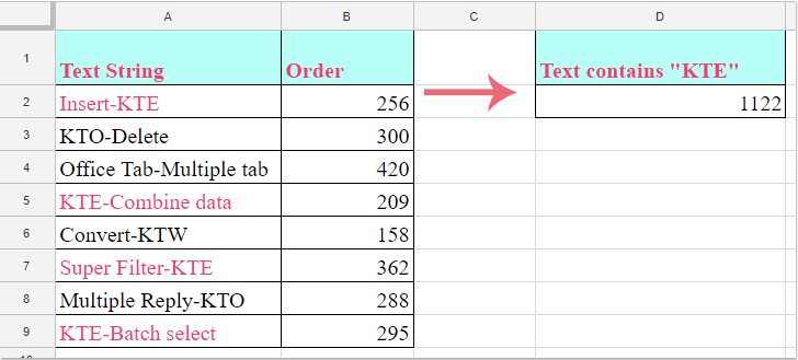
I grynhoi gwerthoedd celloedd mewn colofn os yw celloedd colofn arall yn cynnwys rhan o linyn testun penodol fel a ganlyn y llun a ddangosir, bydd yr erthygl hon yn cyflwyno rhywfaint o fformiwla ddefnyddiol i ddatrys y dasg hon yn nhaflenni Google.

mae doc sumif yn cynnwys testun 1

Celloedd Sumif os yw'n cynnwys rhan o linyn testun penodol yn nhaflenni Google gyda fformwlâu


Celloedd Sumif os yw'n cynnwys rhan o linyn testun penodol yn nhaflenni Google gyda fformwlâu

Gall y fformwlâu canlynol eich helpu i grynhoi gwerthoedd celloedd os yw celloedd colofn arall yn cynnwys llinyn testun penodol, gwnewch hyn:

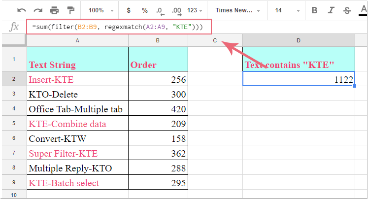
1. Rhowch y fformiwla hon: =sum(filter(B2:B9, regexmatch(A2:A9, "KTE"))) i mewn i gell wag, ac yna pwyswch Rhowch allwedd i gael y canlyniad, gweler y screenshot:

mae doc sumif yn cynnwys testun 2

Nodiadau:

1. Yn y fformiwla uchod: B2: B9 yw'r gwerthoedd celloedd rydych chi am eu crynhoi, A2: A9 ydy'r ystod yn cynnwys y llinyn testun penodol, “KTE”Yw'r testun penodol rydych chi am ei grynhoi yn seiliedig, newidiwch nhw i'ch angen.

2. Dyma fformiwla arall a all eich helpu hefyd: =sumif(A2:A9,"*KTE*",B2:B9).

Offer Cynhyrchiant Swyddfa Gorau

🤖 Kutools AI Aide: Chwyldro dadansoddi data yn seiliedig ar: Cyflawniad Deallus   |  Cynhyrchu Cod  |  Creu Fformiwlâu Personol  |  Dadansoddi Data a Chynhyrchu Siartiau  |  Invoke Swyddogaethau Kutools...
Nodweddion Poblogaidd: Darganfod, Amlygu neu Adnabod Dyblygiadau   |  Dileu Rhesi Gwag   |  Cyfuno Colofnau neu Gelloedd heb Colli Data   |   Rownd heb Fformiwla ...
Super-edrych: VLookup Meini Prawf Lluosog    VLookup Gwerth Lluosog  |   VLookup Ar Draws Taflenni Lluosog   |   Edrych Niwlog ....
Rhestr gwympo Uwch: Creu Rhestr Gollwng yn Gyflym   |  Rhestr Gollwng Dibynnol   |  Rhestr Gollwng Aml-ddewis ....
Rheolwr Colofn: Ychwanegu Nifer Penodol o Golofnau  |  Symud Colofnau  |  Toglo Statws Gwelededd Colofnau Cudd  |  Cymharwch Ystodau a Cholofnau ...
Nodweddion dan Sylw: Ffocws ar y Grid   |  Golwg Dylunio   |   Bar Fformiwla Mawr    Rheolwr Llyfr Gwaith a Thaflen   |  Llyfrgell Adnoddau (Testun Auto)   |  Dewiswr Dyddiad   |  Cyfuno Taflenni Gwaith   |  Amgryptio/Dadgryptio Celloedd    Anfon E-byst trwy Restr   |  Hidlo Super   |   Hidlo Arbennig (hidlo mewn print trwm/italig/strikethrough...) ...
15 Set Offer Gorau12 Testun offer (Ychwanegu Testun, Dileu Cymeriadau,...)   |   50 + Siart Mathau (Siart Gantt,...)   |   40+ Ymarferol Fformiwlâu (Cyfrifwch oedran yn seiliedig ar ben-blwydd,...)   |   19 mewnosod offer (Mewnosod Cod QR, Mewnosod Llun o'r Llwybr,...)   |   12 Trosi offer (Rhifau i Eiriau, Trosi arian cyfred,...)   |   7 Uno a Hollti offer (Rhesi Cyfuno Uwch, Celloedd Hollt,...)   |   ... a mwy

Supercharge Eich Sgiliau Excel gyda Kutools ar gyfer Excel, a Phrofiad Effeithlonrwydd Fel Erioed Erioed. Kutools ar gyfer Excel Yn Cynnig Dros 300 o Nodweddion Uwch i Hybu Cynhyrchiant ac Arbed Amser.  Cliciwch Yma i Gael Y Nodwedd Sydd Ei Angen Y Mwyaf...

Disgrifiad


Mae Office Tab yn dod â rhyngwyneb Tabbed i Office, ac yn Gwneud Eich Gwaith yn Haws o lawer

  • Galluogi golygu a darllen tabbed yn Word, Excel, PowerPoint, Cyhoeddwr, Mynediad, Visio a Phrosiect.
  • Agor a chreu dogfennau lluosog mewn tabiau newydd o'r un ffenestr, yn hytrach nag mewn ffenestri newydd.
  • Yn cynyddu eich cynhyrchiant 50%, ac yn lleihau cannoedd o gliciau llygoden i chi bob dydd!
Comments (9)
No ratings yet. Be the first to rate!
This comment was minimized by the moderator on the site
Hello, Thank for super post. I had was able to solve few issues with it. I still have one issue isuse- I am unable to sum up if there is a number in condition column say "=SUMIF(B9:B2414;"85*";E9:E2414)" where B can contains values like "ABC", "851", "865", "LUX",etc.
This comment was minimized by the moderator on the site
Hello !
Thank you for this tuto.

Is it possible to sum numbers included in cells if those cells also include a specific word ?

For example :
"car 2"
"house 1"
"dog 7"
"plate 3"
"screen 4"
"horse 2"
"battery 9"
"floor 1"
"river 2"
"plane 0"
"butterfly 7"
"horse 1"
"plate 0"
"house 12"

Formula to find total of house ?
Answer in this examle is 13

"house 1" is the content of one cell. I can't transfer the content in to different cells.
Thank you for your help.

https://i.postimg.cc/26LrtGNt/sumif.jpg
This comment was minimized by the moderator on the site
Thanks for this. I found both techniques shown work, EXCEPT that the filter and regex method returns an N/A error if there are not matches to the filter. So when I have a number of these formulas in a column and then sum the total, using that method causes the sum to return N/A and therefore the totals to break.  However using the sumif and *KTE* method returns a sum of 0 if there are no results, so the summing of totals still works. 
This comment was minimized by the moderator on the site
Hello jodamo5,I get your point. Indeed, the filter and regex method returns an #N/A error when there are no matches to filter. Therefore, I recommend the sumif method. Thanks for your notice. Your support means a lot to us. Have a great day.Sincerely,Mandy
This comment was minimized by the moderator on the site
Hey,
If I want to sum based on one of TWO specific text strains: Ex - "KTE" OR "ABC", would that be possible?
This comment was minimized by the moderator on the site
Hello, Adam,To sum the values based on more specifc text, any of the following formulas can do you a favor.=SUMIF(A2:A7, "*KTE*", B2:B7)+SUMIF(A2:A7, "*ABC*", B2:B7)
=sum(filter(B2:B7, regexmatch(A2:A7, "KTE")))+sum(filter(B2:B7, regexmatch(A2:A7, "ABC")))
please try, hope it can help you!
This comment was minimized by the moderator on the site
Hi,

the sum if formular is really useful. However, do you know how to make the text string dynamic (meaning referring to a cell)?

E.g. "*KTE*" replaced with something like C2 if the text string is in column C already.

=sumif(A2:A9,"*KTE*",B2:B9).
This comment was minimized by the moderator on the site
Hi, Sunith,
To replace the specific text with cell reference, please apply the below formula, change the cell C2 to your need.
=sumif(A2:A9,"*"&C2&"*",B2:B9)

Please try, thank you!
This comment was minimized by the moderator on the site
It works - thank you!
There are no comments posted here yet
Please leave your comments in English
Posting as Guest
×
Rate this post:
0   Characters
Suggested Locations