Skip i'r prif gynnwys

Sut i wylio i ddychwelyd colofnau lluosog o dabl Excel?

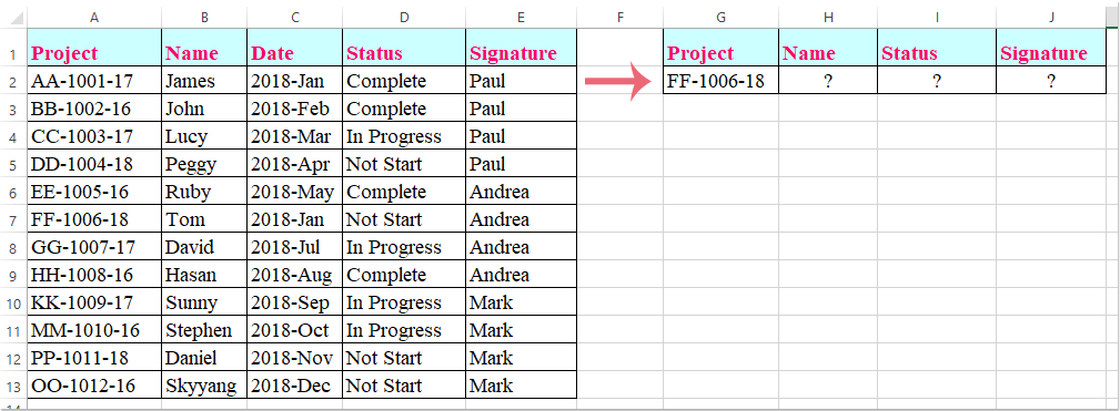
Yn nhaflen waith Excel, gallwch gymhwyso'r swyddogaeth Vlookup i ddychwelyd y gwerth paru o un golofn. Ond, weithiau, efallai y bydd angen i chi dynnu gwerthoedd cyfatebol o sawl colofn fel y dangosir y llun a ganlyn. Sut allech chi gael y gwerthoedd cyfatebol ar yr un pryd o sawl colofn trwy ddefnyddio'r swyddogaeth Vlookup?

col vlookup colofnau lluosog 1

Vlookup i ddychwelyd gwerthoedd paru o golofnau lluosog gyda fformiwla arae


Vlookup i ddychwelyd gwerthoedd paru o golofnau lluosog gyda fformiwla arae

Yma, byddaf yn cyflwyno'r swyddogaeth Vlookup i ddychwelyd gwerthoedd cyfatebol o sawl colofn, gwnewch fel hyn:

1. Dewiswch y celloedd lle rydych chi am roi'r gwerthoedd paru o sawl colofn, gweler y screenshot:

col vlookup colofnau lluosog 2

2. Yna nodwch y fformiwla hon: =VLOOKUP(G2,A1:E13,{2,4,5},FALSE) i mewn i'r bar fformiwla, ac yna pwyswch Ctrl + Shift + Enter mae allweddi gyda'i gilydd, ac mae'r gwerthoedd paru o golofnau lluosog wedi'u tynnu ar unwaith, gweler y screenshot:

col vlookup colofnau lluosog 3

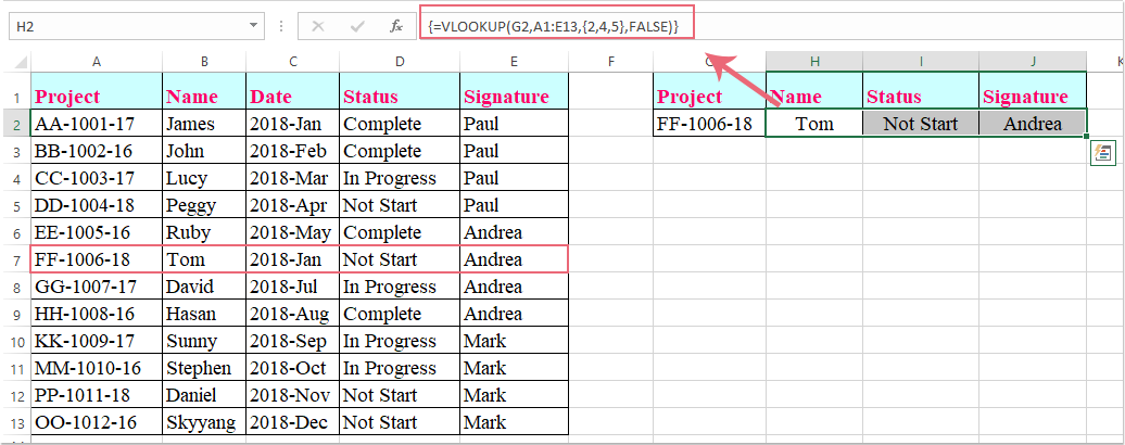
Nodyn: Yn y fformiwla uchod, G2 yw'r meini prawf rydych chi am ddychwelyd gwerthoedd yn seiliedig ar, A1: E13 yw'r ystod bwrdd rydych chi am edrych arno, y rhif 2, 4, 5 yw'r rhifau colofn yr ydych am ddychwelyd gwerthoedd ohonynt.

Offer Cynhyrchiant Swyddfa Gorau

🤖 Kutools AI Aide: Chwyldro dadansoddi data yn seiliedig ar: Cyflawniad Deallus   |  Cynhyrchu Cod  |  Creu Fformiwlâu Personol  |  Dadansoddi Data a Chynhyrchu Siartiau  |  Invoke Swyddogaethau Kutools...
Nodweddion Poblogaidd: Darganfod, Amlygu neu Adnabod Dyblygiadau   |  Dileu Rhesi Gwag   |  Cyfuno Colofnau neu Gelloedd heb Colli Data   |   Rownd heb Fformiwla ...
Super-edrych: VLookup Meini Prawf Lluosog    VLookup Gwerth Lluosog  |   VLookup Ar Draws Taflenni Lluosog   |   Edrych Niwlog ....
Rhestr gwympo Uwch: Creu Rhestr Gollwng yn Gyflym   |  Rhestr Gollwng Dibynnol   |  Rhestr Gollwng Aml-ddewis ....
Rheolwr Colofn: Ychwanegu Nifer Penodol o Golofnau  |  Symud Colofnau  |  Toglo Statws Gwelededd Colofnau Cudd  |  Cymharwch Ystodau a Cholofnau ...
Nodweddion dan Sylw: Ffocws ar y Grid   |  Golwg Dylunio   |   Bar Fformiwla Mawr    Rheolwr Llyfr Gwaith a Thaflen   |  Llyfrgell Adnoddau (Testun Auto)   |  Dewiswr Dyddiad   |  Cyfuno Taflenni Gwaith   |  Amgryptio/Dadgryptio Celloedd    Anfon E-byst trwy Restr   |  Hidlo Super   |   Hidlo Arbennig (hidlo mewn print trwm/italig/strikethrough...) ...
15 Set Offer Gorau12 Testun offer (Ychwanegu Testun, Dileu Cymeriadau,...)   |   50 + Siart Mathau (Siart Gantt,...)   |   40+ Ymarferol Fformiwlâu (Cyfrifwch oedran yn seiliedig ar ben-blwydd,...)   |   19 mewnosod offer (Mewnosod Cod QR, Mewnosod Llun o'r Llwybr,...)   |   12 Trosi offer (Rhifau i Eiriau, Trosi arian cyfred,...)   |   7 Uno a Hollti offer (Rhesi Cyfuno Uwch, Celloedd Hollt,...)   |   ... a mwy

Supercharge Eich Sgiliau Excel gyda Kutools ar gyfer Excel, a Phrofiad Effeithlonrwydd Fel Erioed Erioed. Kutools ar gyfer Excel Yn Cynnig Dros 300 o Nodweddion Uwch i Hybu Cynhyrchiant ac Arbed Amser.  Cliciwch Yma i Gael Y Nodwedd Sydd Ei Angen Y Mwyaf...

Disgrifiad


Mae Office Tab yn dod â rhyngwyneb Tabbed i Office, ac yn Gwneud Eich Gwaith yn Haws o lawer

  • Galluogi golygu a darllen tabbed yn Word, Excel, PowerPoint, Cyhoeddwr, Mynediad, Visio a Phrosiect.
  • Agor a chreu dogfennau lluosog mewn tabiau newydd o'r un ffenestr, yn hytrach nag mewn ffenestri newydd.
  • Yn cynyddu eich cynhyrchiant 50%, ac yn lleihau cannoedd o gliciau llygoden i chi bob dydd!
Comments (15)
No ratings yet. Be the first to rate!
This comment was minimized by the moderator on the site
how can i search for multiple lookup value?for eg: these two arrays shows diff freq coumn,gain,veritcal BW,tolerance etc.I want to get an average values gain and 3db BW..how can i enter the formula
y1    1800    7.5dBi +/- 2.9    22.1° +/- 6.8        7.5
y1    1900    7.6dBi +/- 3.0    18.9° +/- 3.6        7.6
y1    2100    6.7dBi +/- 2.6    17.7° +/- 3.6        6.7
y1    AWS    7.2dBi +/- 2.8    20.4° +/- 9.4        7.2
y1    2300    8.3dBi +/- 3.6    15.8° +/- 1.6        8.3
y1    2600    7.9dBi +/- 2.4    17.1° +/- 1.7        7.9
y2    1800    6.9dBi +/- 1.4    27.1° +/- 10.8        6.9
y2    1900    6.9dBi +/- 1.5    23.0° +/- 12.5        6.9
y2    2100    7.6dBi +/- 2.3    21.7° +/- 19.6        7.6
y2    AWS    8.0dBi +/- 2.5    23.3° +/- 13.8        8
y2    2300    7.7dBi +/- 1.6    15.9° +/- 5.9        7.7
y2    2600    6.5dBi +/- 2.3    14.5° +/- 3.9        6.5
This comment was minimized by the moderator on the site
I have many rows with same value but need to get multiple value after look up, I need to get two different EO ref , how can U##TRX EO
HXPRE-MQ1371 AB0024822
This comment was minimized by the moderator on the site
Thank you!! The { } of the columns is what I was missing. Appreciate this page!
This comment was minimized by the moderator on the site
Thanks! Super helpful, when other online options weren't
This comment was minimized by the moderator on the site
What if you need to have multiple rows as well? Ex. find all the FF-1006-18 rows while still only bringing back column B, D, and E.
This comment was minimized by the moderator on the site
Hello, Shelly,
Maybe there is not a direct formula for helping you, but, you can apply the below array fromula to get all matching values from the entire row, and then delete or hide the unwanted column as you need.
=INDEX($A$2:$E$10, SMALL(IF($G$2=$A$2:$A$10, ROW($A$2:$A$10)-MIN(ROW($A$2:$A$10))+1, ""), ROW(B1)),COLUMN(B1))
Then press Ctrl + Shift + Enter keys to get the first cell and then drag the fill handle to right and then drga down to get all corresponding values.

Please try, hope it can help you!
This comment was minimized by the moderator on the site
Thanks! This was really Helpful!
This comment was minimized by the moderator on the site
This method does not work. Even if it did, it is not the proper method.
Example of correct method is:
VLOOKUP($A2:$A1093, '[Workbook1.xlsx]Sheet2'!$A$2:$D$111,COLUMN(G2),FALSE)

Make sure you add $ before the column letter of your lookup reference to make sure it remains static, once done, using the filler button on the selected target cell, drag right to the corresponding number of columns.
This comment was minimized by the moderator on the site
This comment is exactly what I needed
This comment was minimized by the moderator on the site
How can I do this using 2 different spread sheets?
This comment was minimized by the moderator on the site
Hello, Lana,
The above formula in this article also can help you to get the results in another worksheet, you just need to change the cell reference as follows:
=VLOOKUP(A1,Sheet1!A1:E13,{2,4,5},FALSE)
Please remember to press Ctrl + Shift + Enter keys together to get the correct results.
This comment was minimized by the moderator on the site
NOT GETTING MULTIPLE COLUMN I'M GETTING ONLY ONE COLUMN VALUE
This comment was minimized by the moderator on the site
Hi, HARI,
To apply this formula, first, you should select the multiple cells where you want to output the results, and then copy the formula into the formula bar, then press Ctrl + Shift + Enter keys together to get the results.
Please try, hope it can help you!
This comment was minimized by the moderator on the site
This is great. How do I carry this formula down if I have 10,000 rows? I've tried a few ways but of course it's changing the formula on me.
This comment was minimized by the moderator on the site
Hi, Scully,
To apply this formula to multiple rows, you just need to change the relative cell reference to absolute reference, as this: =VLOOKUP(A1,Sheet1!$A$1:$E$13,{2,4,5},FALSE).
Please try this, hope it can help you!
There are no comments posted here yet
Please leave your comments in English
Posting as Guest
×
Rate this post:
0   Characters
Suggested Locations