Skip i'r prif gynnwys

Sut i ddychwelyd gwerthoedd paru lluosog yn seiliedig ar un neu feini prawf lluosog yn Excel?

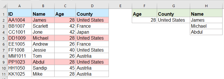
Fel rheol, mae'n hawdd i'r mwyafrif ohonom edrych ar werth penodol a dychwelyd yr eitem baru trwy ddefnyddio'r swyddogaeth VLOOKUP. Ond, a ydych erioed wedi ceisio dychwelyd gwerthoedd paru lluosog yn seiliedig ar un neu fwy o feini prawf fel a ddangosir y screenshot canlynol? Yn yr erthygl hon, byddaf yn cyflwyno rhai fformiwlâu ar gyfer datrys y dasg gymhleth hon yn Excel.

Dychwelwch werthoedd paru lluosog yn seiliedig ar un neu fwy o feini prawf gyda fformwlâu arae


Dychwelwch werthoedd paru lluosog yn seiliedig ar un neu fwy o feini prawf gyda fformwlâu arae

Er enghraifft, rwyf am dynnu pob enw y mae ei oedran yn 28 oed ac sy'n dod o'r Unol Daleithiau, cymhwyswch y fformiwla ganlynol:

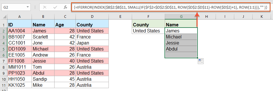
1. Copïwch neu nodwch y fformiwla isod mewn cell wag lle rydych chi am ddod o hyd i'r canlyniad:

=INDEX($B$2:$B$11, SMALL(IF(COUNTIF($F$2, $C$2:$C$11)*COUNTIF($G$2, $D$2:$D$11), ROW($A$2:$D$11)-MIN(ROW($A$2:$D$11))+1), ROW(A1)), COLUMN(A1))

Nodyn: Yn y fformiwla uchod, B2: B11 yw'r golofn y dychwelir y gwerth paru ohoni; F2, C2: C11 yw'r cyflwr cyntaf a'r data colofn sy'n cynnwys yr amod cyntaf; G2, D2: D11 yw'r ail amod a'r data colofn sy'n cynnwys yr amod hwn, newidiwch nhw i'ch angen.

2. Yna, pwyswch Ctrl + Shift + Enter allweddi i gael y canlyniad paru cyntaf, ac yna dewiswch y gell fformiwla gyntaf a llusgwch y ddolen llenwi i lawr i'r celloedd nes bod gwerth gwall yn cael ei arddangos, nawr, dychwelir yr holl werthoedd paru fel y dangosir isod y llun:

Awgrymiadau: Os oes angen i chi ddychwelyd yr holl werthoedd paru yn seiliedig ar un amod, defnyddiwch y fformiwla arae isod:

=IFERROR(INDEX($B$2:$B$11, SMALL(IF($F$2=$D$2:$D$11, ROW($D$2:$D$11)-ROW($D$2)+1), ROW(1:1))),"" )


Erthyglau mwy cymharol:

  • Dychwelwch Werthoedd Edrych Lluosog Mewn Un Gell sydd wedi'i Gwahanu â Choma
  • Yn Excel, gallwn gymhwyso swyddogaeth VLOOKUP i ddychwelyd y gwerth cyfatebol cyntaf o gelloedd bwrdd, ond, weithiau, mae angen i ni dynnu'r holl werthoedd paru ac yna eu gwahanu gan amffinydd penodol, fel coma, dash, ac ati ... i mewn i un cell fel y dangosir y screenshot canlynol. Sut y gallem gael a dychwelyd gwerthoedd edrych lluosog mewn un gell sydd wedi'i gwahanu gan goma yn Excel?
  • Vlookup A Dychwelyd Gwerthoedd Paru Lluosog Ar Unwaith Yn Nhaflen Google
  • Gall y swyddogaeth Vlookup arferol yn nhaflen Google eich helpu i ddod o hyd i'r gwerth paru cyntaf a'i ddychwelyd yn seiliedig ar ddata penodol. Ond, weithiau, efallai y bydd angen i chi wylio a dychwelyd yr holl werthoedd paru fel y dangosir y llun a ddangosir. A oes gennych unrhyw ffyrdd da a hawdd o ddatrys y dasg hon ar ddalen Google?
  • Vlookup A Dychwelyd Gwerthoedd Lluosog O'r Rhestr Gostwng
  • Yn Excel, sut allech chi wylio a dychwelyd sawl gwerth cyfatebol o gwymplen, sy'n golygu pan fyddwch chi'n dewis un eitem o'r gwymplen, mae ei holl werthoedd cymharol yn cael eu harddangos ar unwaith fel y dangosir y screenshot canlynol. Yr erthygl hon, byddaf yn cyflwyno'r datrysiad gam wrth gam.
  • Vlookup A Dychwelyd Gwerthoedd Lluosog yn Fertigol Yn Excel
  • Fel rheol, gallwch ddefnyddio'r swyddogaeth Vlookup i gael y gwerth cyfatebol cyntaf, ond, weithiau, rydych chi am ddychwelyd yr holl gofnodion paru yn seiliedig ar faen prawf penodol. Yr erthygl hon, byddaf yn siarad am sut i wylio a dychwelyd yr holl werthoedd paru yn fertigol, yn llorweddol neu i mewn i un gell.
  • Vlookup A Dychwelyd Data Paru Rhwng Dau Werth Yn Excel
  • Yn Excel, gallwn gymhwyso'r swyddogaeth Vlookup arferol i gael y gwerth cyfatebol yn seiliedig ar ddata penodol. Ond, weithiau, rydyn ni am wylio a dychwelyd y gwerth paru rhwng dau werth fel y dangosir y screenshot canlynol, sut allech chi ddelio â'r dasg hon yn Excel?


  • Bar Fformiwla Gwych (golygu llinellau lluosog o destun a fformiwla yn hawdd); Cynllun Darllen (darllen a golygu nifer fawr o gelloedd yn hawdd); Gludo i'r Ystod Hidlo...
  • Uno Celloedd / Rhesi / Colofnau a Cadw Data; Cynnwys Celloedd Hollt; Cyfuno Rhesi Dyblyg a Swm / Cyfartaledd... Atal Celloedd Dyblyg; Cymharwch y Meysydd...
  • Dewiswch Dyblyg neu Unigryw Rhesi; Dewiswch Blank Rows (mae pob cell yn wag); Darganfyddiad Gwych a Darganfyddiad Niwlog mewn Llawer o Lyfrau Gwaith; Dewis ar Hap ...
  • Copi Union Celloedd Lluosog heb newid cyfeirnod fformiwla; Auto Creu Cyfeiriadau i Daflenni Lluosog; Mewnosod Bwledi, Blychau Gwirio a mwy ...
  • Fformiwlâu Hoff a Mewnosod yn Gyflym, Meysydd, Siartiau a Lluniau; Amgryptio Celloedd gyda chyfrinair; Creu Rhestr Bostio ac anfon e-byst ...
  • Testun Detholiad, Ychwanegu Testun, Tynnu yn ôl Swydd, Tynnwch y Gofod; Creu ac Argraffu Subtotals Paging; Trosi rhwng Cynnwys a Sylwadau Celloedd...
  • Hidlo Super (arbed a chymhwyso cynlluniau hidlo i ddalenni eraill); Trefnu Uwch yn ôl mis / wythnos / dydd, amlder a mwy; Hidlo Arbennig gan feiddgar, italig ...
  • Cyfuno Llyfrau Gwaith a Thaflenni Gwaith; Uno Tablau yn seiliedig ar golofnau allweddol; Rhannwch Ddata yn Daflenni Lluosog; Trosi Swp xls, xlsx a PDF...
  • Grwpio Tabl Pivot yn ôl rhif wythnos, diwrnod o'r wythnos a mwy ... Dangos Celloedd Datgloi, wedi'u Cloi yn ôl gwahanol liwiau; Amlygu Celloedd sydd â Fformiwla / Enw...
tab kte 201905
  • Galluogi golygu a darllen tabbed yn Word, Excel, PowerPoint, Cyhoeddwr, Mynediad, Visio a Phrosiect.
  • Agor a chreu dogfennau lluosog mewn tabiau newydd o'r un ffenestr, yn hytrach nag mewn ffenestri newydd.
  • Yn cynyddu eich cynhyrchiant 50%, ac yn lleihau cannoedd o gliciau llygoden i chi bob dydd!
gwaelod officetab


Comments (25)
No ratings yet. Be the first to rate!
This comment was minimized by the moderator on the site
Hi, if there are duplicate values (e.g. two adams), how do i make sure that it only returns 1 adam and not 2?
This comment was minimized by the moderator on the site
Hello, Bobby,
To extract only unique matching values, you should apply the below formula:
After pasting the formula, please press Ctrl + Shift + Enter keys together to get the correct result.
=IFERROR(INDEX($B$2:$B$5, MATCH(0, COUNTIF(H1:$H$1, $B$2:$B$5)+IF($D$2:$D$5<>$G$2, 1, 0)+IF($C$2:$C$5<>$F$2, 1, 0), 0)), "")

Please have a try, hope it can help you!
This comment was minimized by the moderator on the site
Hi,

Thanks for posting these examples.
I'm trying to implement this in my own sheet, but don't get it to work (maybe because I'm using an europe version of excel)?

I want to get the dates of the days that I had my shifts or that I have worked 'some' (>0) hours for a client.

So in I3 is the name and in J3 the month. K3 and L3 are the shifts (1 is worked) and hours (don't know how to set this, should be more than zero)

My expected results are in:
Shifts: I7 and I8
hours: J7

So I worked more than 0 hours for 'person 2' in oktober on 3-10-2022
had shifts for person 2 on '10-10-2022' and 28-10-2022

When I add '=INDEX($B$2:$B$11, SMALL(IF(COUNTIF($F$2, $C$2:$C$11)*COUNTIF($G$2, $D$2:$D$11), ROW($A$2:$D$11)-MIN(ROW($A$2:$D$11))+1), ROW(A1)), COLUMN(A1))' in my excel sheet, it doesn't allow the comma between the different parts of the formula.
So I need to change them to ';'.
But when I try it it always says: '#NAME?'

So can someone help me with this?

Kind regards,

Bas
[img]https://drive.google.com/file/d/1iIPQKuj_PNhqWyWlwJ4IQTqGNEd6B9Hw/view?usp=share_link[/img]
This comment was minimized by the moderator on the site
Hi,

First, thank you for sharing!

Can you please provide a solution to the case below:

I have 3 columns (A: Containing reference information, B: Containing information to be searched, C: Search result)

Image url is provided below

https://ibb.co/VHCd09K

Column A-------------------------Column B------------Column C
File Name-------------------------Name----------------File Name, Document Name, Element Name, Name
Changed Element-----------------Element--------------Changed Element, Element Name, Element ID
Column Location
Document Name
Element Name
Name
Category
Warranty
Slope
Element ID

What I need is to search in column A for any partial match with cell B2 (Name) or B3 (Element) and get the result in one cell,

Thank you, Behzad
This comment was minimized by the moderator on the site
Hello, Behzad
Maybe the below User Defined Function can help you.
Public Function ConcatPartLookUp(rngInput As Range, rngSource As Range, Optional strDelimiter As String, Optional blCaseSensitive)
Dim rng As Range
If strDelimiter = "" Then strDelimiter = ","
If IsMissing(blCaseSensitive) Then
    blCaseSensitive = False
Else
    blCaseSensitive = True
End If
For Each rng In rngSource
    If blCaseSensitive Then
        If InStr(1, rng.Value, rngInput.Value, vbBinaryCompare) > 0 Then ConcatPartLookUp = ConcatPartLookUp & strDelimiter & rng.Value
    Else
        If InStr(1, rng.Value, rngInput.Value, vbTextCompare) > 0 Then ConcatPartLookUp = ConcatPartLookUp & strDelimiter & rng.Value
    End If
Next
If Len(ConcatPartLookUp) > 0 Then ConcatPartLookUp = Mid(ConcatPartLookUp, 2, Len(ConcatPartLookUp))
End Function


After copying and pasting this code, and then use this formula:=ConcatPartLookUp(B2,$A$2:$A$8) to get the result you need.
Please have a try, hope it can help you!
This comment was minimized by the moderator on the site
Heyi, thank you for the formula. It worked for "fixed" values / text as criterias. However, one of the criterias i'm trying to use is a condition (values <>0 ), but does not work the described formula. Do you guys know what should i change to adapt the formula so I can have a condition as one of the criterias, please?

Best,

João
This comment was minimized by the moderator on the site
Hello, Marcus
To solve your problem, please view this article:
https://www.extendoffice.com/documents/excel/6393-excel-vlookup-function.html#b3-2
There are some detailed explanations of this task. You just need to change the criteira to your own.
Thank you!
This comment was minimized by the moderator on the site
Hi,

if in cell H1 i write "Name" and wanted to link that with the formula, how would that work?
Then I could write "ID" in cell H1 and would automatically get as a result: AA1004; DD1009; PP1023 (for the first formula)

Thank you in advance!
This comment was minimized by the moderator on the site
Hello, Marie
Sorry, i can't get the point of your first problem, could you explain your problem more clearly and detailedly? Or you can insert a screenshot here to describe your problem.
As for the second question, you just need to change the cell reference as this:
=INDEX($A$2:$A$11, SMALL(IF(COUNTIF($F$2, $C$2:$C$11)*COUNTIF($G$2, $D$2:$D$11), ROW($A$2:$D$11)-MIN(ROW($A$2:$D$11))+1), ROW(A1)), COLUMN(A1))

Remeber to press Ctrl + Shift + Enter keys together.
Please try, hope it can help you!
This comment was minimized by the moderator on the site
Hello,
what would be needed to expand the first formula in the following case:
Some IDs are Blank (e.g. cell A5 is blank) and I would like an additional condition outputting lines only when the IDs are not blank. (So the output should then be James and Abdul.
Thanks!
This comment was minimized by the moderator on the site
Hello, Jo,
To solve your problem, please apply the below formula:
=INDEX($B$2:$B$11, SMALL(IF(COUNTIF($F$2, $C$2:$C$11)*COUNTIF($G$2, $D$2:$D$11)*($A$2:$A$11<>0), ROW($A$2:$D$11)-MIN(ROW($A$2:$D$11))+1), ROW(A1)), COLUMN(A1))

Please have a ry, hope it can help you!
This comment was minimized by the moderator on the site
hello,
ive tried using the formula and it either generates a value of 0 or the image attached
This comment was minimized by the moderator on the site
Hello, Milku
Your screenshot showed WPS software of MAC version, so I am not sure whether our formula is available.
I uploaded an Excel file to here, you can try to see if it can calculate correctly in you environment.
Thank you!
This comment was minimized by the moderator on the site
When I use the second formula and drag down, nothing appears. The formula result (fx) says it should be returning something but it is blank. How do I correct this?
This comment was minimized by the moderator on the site
Hello Alysia,

Glad to help. I tried the second formula in the article and drag the formula down, the rest of results were returned. I think there may be two reasons for your problem. First, maybe you forget to press Ctrl + Shift + Enter keys to enter the formula. Second, the matching result is only one, so no other results are not returned. Please have a check.

Sincerely,
Mandy
This comment was minimized by the moderator on the site
Hi,

I was wondering if it at all possible to enter a 2nd criteria but from the same range as the 1st criteria,

For example with the used example above i would like to search for the names of people from both America and France So cell F3 would have France, Scarlett & Andrew would also populate in the list in Column G

Thank you for assistance in advance.
This comment was minimized by the moderator on the site
Hello Nick,

Glad to help. If you want to get the names of people from both America and France, I advise you to use our formula twice to get the result. Please see the screenshot, In F2 and G2 are values "United States" and "France". Apply formula =IFERROR(INDEX($B$2:$B$11, SMALL(IF($F$2=$D$2:$D$11, ROW($D$2:$D$11)-ROW($D$2)+1), ROW(1:1))),"" ) to get the results for America. And apply formula =IFERROR(INDEX($B$2:$B$11, SMALL(IF($G$2=$D$2:$D$11, ROW($D$2:$D$11)-ROW($D$2)+1), ROW(1:1))),"" ) to get the results for France. It's simple. Please have a try.

Sincerely,
Mandy
This comment was minimized by the moderator on the site
In the first example, what change to the formula would be needed to return everyone who was less than 28 years old?
There are no comments posted here yet
Load More
Please leave your comments in English
Posting as Guest
×
Rate this post:
0   Characters
Suggested Locations