Skip i'r prif gynnwys

Sut i ddod o hyd i ddydd Gwener cyntaf neu ddydd Gwener olaf pob mis yn Excel?

Awdur: Siluvia Wedi'i Addasu Diwethaf: 2020-07-22

Fel rheol dydd Gwener yw'r diwrnod gwaith olaf mewn mis. Sut allwch chi ddod o hyd i'r dydd Gwener cyntaf neu'r dydd Gwener diwethaf yn seiliedig ar ddyddiad penodol yn Excel? Yn yr erthygl hon, byddwn yn eich tywys trwy sut i ddefnyddio dau fformiwla ar gyfer dod o hyd i'r dydd Gwener cyntaf neu'r dydd Gwener olaf o bob mis.

Dewch o hyd i'r dydd Gwener cyntaf o fis
Dewch o hyd i'r dydd Gwener olaf o fis


Dewch o hyd i'r dydd Gwener cyntaf o fis

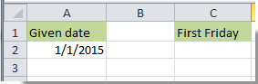
Er enghraifft, mae dyddiad penodol 1/1/2015 yn lleoli yng nghell A2 fel y dangosir isod y screenshot. Os ydych chi am ddod o hyd i ddydd Gwener cyntaf y mis yn seiliedig ar y dyddiad penodol, gwnewch fel a ganlyn.

1. Dewiswch gell i arddangos y canlyniad. Yma rydym yn dewis y gell C2.

2. Copïwch a gludwch y fformiwla isod i mewn iddi, yna pwyswch y Rhowch allweddol.

=CEILING(EOMONTH(A2,-1)-5,7)+6

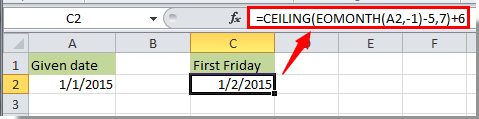
Yna mae'r dyddiad yn cael ei arddangos yng nghell C2, mae'n golygu mai dydd Gwener cyntaf Ionawr 2015 yw'r dyddiad 1/2/2015.

Nodiadau:

1. Os ydych chi am ddod o hyd i ddydd Gwener cyntaf misoedd eraill, nodwch y dyddiad penodedig y mis hwnnw yng nghell A2, ac yna defnyddiwch y fformiwla.

2. Yn y fformiwla, A2 yw'r gell gyfeirio y mae'r dyddiad penodol yn ei lleoli. Gallwch ei newid i ddiwallu'ch anghenion.

Dewch o hyd i'r dydd Gwener olaf o fis

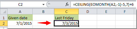
Mae'r dyddiad penodol 1/1/2015 yn lleoli yng nghell A2, ar gyfer dod o hyd i ddydd Gwener olaf y mis hwn yn Excel, gwnewch fel a ganlyn.

1. Dewiswch gell, copïwch y fformiwla isod i mewn iddi, ac yna pwyswch y Rhowch allwedd i gael y canlyniad.

=DATE(YEAR(A2),MONTH(A2)+1,0)+MOD(-WEEKDAY(DATE(YEAR(A2),MONTH(A2)+1,0),2)-2,-7)

Yna mae dydd Gwener olaf mis Ionawr 2015 yn arddangos y gell B2.

Nodyn: Gallwch newid A2 yn y fformiwla i gell gyfeirio eich dyddiad penodol.


Erthyglau cysylltiedig:

Offer Cynhyrchiant Swyddfa Gorau

🤖 Kutools AI Aide: Chwyldro dadansoddi data yn seiliedig ar: Cyflawniad Deallus   |  Cynhyrchu Cod  |  Creu Fformiwlâu Personol  |  Dadansoddi Data a Chynhyrchu Siartiau  |  Invoke Swyddogaethau Kutools...
Nodweddion Poblogaidd: Darganfod, Amlygu neu Adnabod Dyblygiadau   |  Dileu Rhesi Gwag   |  Cyfuno Colofnau neu Gelloedd heb Colli Data   |   Rownd heb Fformiwla ...
Super-edrych: VLookup Meini Prawf Lluosog    VLookup Gwerth Lluosog  |   VLookup Ar Draws Taflenni Lluosog   |   Edrych Niwlog ....
Rhestr gwympo Uwch: Creu Rhestr Gollwng yn Gyflym   |  Rhestr Gollwng Dibynnol   |  Rhestr Gollwng Aml-ddewis ....
Rheolwr Colofn: Ychwanegu Nifer Penodol o Golofnau  |  Symud Colofnau  |  Toglo Statws Gwelededd Colofnau Cudd  |  Cymharwch Ystodau a Cholofnau ...
Nodweddion dan Sylw: Ffocws ar y Grid   |  Golwg Dylunio   |   Bar Fformiwla Mawr    Rheolwr Llyfr Gwaith a Thaflen   |  Llyfrgell Adnoddau (Testun Auto)   |  Dewiswr Dyddiad   |  Cyfuno Taflenni Gwaith   |  Amgryptio/Dadgryptio Celloedd    Anfon E-byst trwy Restr   |  Hidlo Super   |   Hidlo Arbennig (hidlo mewn print trwm/italig/strikethrough...) ...
15 Set Offer Gorau12 Testun offer (Ychwanegu Testun, Dileu Cymeriadau,...)   |   50 + Siart Mathau (Siart Gantt,...)   |   40+ Ymarferol Fformiwlâu (Cyfrifwch oedran yn seiliedig ar ben-blwydd,...)   |   19 mewnosod offer (Mewnosod Cod QR, Mewnosod Llun o'r Llwybr,...)   |   12 Trosi offer (Rhifau i Eiriau, Trosi arian cyfred,...)   |   7 Uno a Hollti offer (Rhesi Cyfuno Uwch, Celloedd Hollt,...)   |   ... a mwy

Supercharge Eich Sgiliau Excel gyda Kutools ar gyfer Excel, a Phrofiad Effeithlonrwydd Fel Erioed Erioed. Kutools ar gyfer Excel Yn Cynnig Dros 300 o Nodweddion Uwch i Hybu Cynhyrchiant ac Arbed Amser.  Cliciwch Yma i Gael Y Nodwedd Sydd Ei Angen Y Mwyaf...

Disgrifiad


Mae Office Tab yn dod â rhyngwyneb Tabbed i Office, ac yn Gwneud Eich Gwaith yn Haws o lawer

  • Galluogi golygu a darllen tabbed yn Word, Excel, PowerPoint, Cyhoeddwr, Mynediad, Visio a Phrosiect.
  • Agor a chreu dogfennau lluosog mewn tabiau newydd o'r un ffenestr, yn hytrach nag mewn ffenestri newydd.
  • Yn cynyddu eich cynhyrchiant 50%, ac yn lleihau cannoedd o gliciau llygoden i chi bob dydd!
Comments (12)
Rated 5 out of 5 · 1 ratings
This comment was minimized by the moderator on the site
Even shorter 😅
=lambda(Date;WeekDay;EOMONTH(Date;0)-WEEKDAY(EOMONTH(Date;0);WeekDay+10)+1
Where "WeekDay" parameter is 1=Monday, 7=Sunday
This comment was minimized by the moderator on the site
=lambda(Date;WeekDay;EOMONTH(Date;0)-WEEKDAY(EOMONTH(Date;0);WeekDay+10)+1)

I forgot a bracket at the end
This comment was minimized by the moderator on the site
Vậy công thức tính thứ sáu tuần thứ 2 của tháng như thế nào vậy ban?
This comment was minimized by the moderator on the site
Hi Tâm Cao Điền,
Suppose you want to calculate the second friday of the month based on the given date in A1, you can try the following formula:
=A18-DAY(A18)+CHOOSE(WEEKDAY(A18-DAY(A18),2),11,10,9,8,14,13,12)
This comment was minimized by the moderator on the site
porque cuando lo pruebo tal cual me sale error ?
o sea estoy copiando y pegando y no funciona

alguien sabe?
This comment was minimized by the moderator on the site
Hi andre,
Can you tell me which formula you used in the post? And what error your are experiencing?
This comment was minimized by the moderator on the site
Why not make the "last Friday" formula: =CEILING(EOMONTH(A2,0)-5,7)-1? That works for all dates I have tried....
This comment was minimized by the moderator on the site
Hi Eric,
I hop you are still on this forum and receive my reply.
Thanks so much for an EASY formula. I've never encountered =CEILING.
Rated 5 out of 5
This comment was minimized by the moderator on the site
Hi Eric,
Thanks for sharing it.
This comment was minimized by the moderator on the site
Hello and thank you for this formula. I am not an Excel guru and acnnot easily work out how to change this formula for the last Friday to be the Last Monday, or any other day. Can you please explain how to interpret this.
This comment was minimized by the moderator on the site
Matt,

The way the formula works is: First we find the last day of the month with the EOMONTH() function. For the last day of the current month, we use "0" as the month offset. For the previous month, it would be -1. (Either "=EOMONTH(A2,0)" or "=EOMONTH(A2,-1)".)

Then, in the "=CEILING()" function, we subtract the number of days required to bring us back to Sunday from the day for which we are searching. (For Tuesday, it would be -2, so we make the formula so far: "=CEILING(EOMONTH(A2,0)-2...."

We use the "significance" value of "7" because weeks are seven days long (of course).This finds the date of either the previous Saturday, or the following Saturday (Excel dates started with 1/1/1900, which was a Sunday. So if you enter a "1" in cell A2 with the Long Date format, the cell would read: "Sunday, January 1, 1900".). For that reason, the =CEILING() function, using "7" as the "significance" argument returns Saturday, which is always a multiple of 7 in Excel. Now the formula is "=CEILING(EOMONTH(A2,0)-2,7...".

Now we need to return the date to a Tuesday, so we either subtract 4 for the last Tuesday of the month, or add 3 for the first Tuesday of the next month. So the final formula is, respectively, either "=CEILING(EOMONTH(A2,0)-2,7)-4" or "=CEILING(EOMONTH(A2,0)-2,7)+3".

We can work through the math by assuming the last day of the month is either a Monday (assume its value is 9 - for ease of illustration, so the values do not go negative) or a Wednesday (assume value 11). "EOMONTH()" will return either of those days (9 or 11). Subtracting 2 results in the previous Saturday (value 7) or Monday (value 9), respectively. The CEILING() function then returns, respectively, the previous Saturday (value 7, because the ceiling of 7 with significance 7 is 7) or the current Saturday (value 14, because the ceiling of 9, significance 7, is 14). Subtracting 4 results in the previous Tuesday (value 3) or the current week's Tuesday (value 10), respectively. For the first Tuesday of the following month, adding 3 to the Saturday value (7 or 14) returns either Tuesday value 10, or Tuesday value 17, respectively.


Hopefully that helps you understand so that you can modify the formula as necessary. You can even change it to find the second Tuesday, or second to last Tuesday, by adding or subtracting an additional 7, respectively.
This comment was minimized by the moderator on the site
Hi Matt,
You just need to change the last number -7 to -1 to solove the problem.
=DATE(YEAR(A2),MONTH(A2)+1,0)+MOD(-WEEKDAY(DATE(YEAR(A2),MONTH(A2)+1,0),2)-2,-1)
There are no comments posted here yet
Please leave your comments in English
Posting as Guest
×
Rate this post:
0   Characters
Suggested Locations