Sut i newid rhifau negyddol i bositif yn Excel?
Pan fyddwch chi'n prosesu gweithrediadau yn Excel, weithiau, efallai y bydd angen i chi newid y rhifau negyddol i'r rhifau positif neu i'r gwrthwyneb. A oes unrhyw driciau cyflym y gallwch wneud cais am newid rhifau negyddol i bositif? Bydd yr erthygl hon yn cyflwyno'r triciau canlynol i chi ar gyfer trosi'r holl rifau negyddol yn bositif neu i'r gwrthwyneb yn hawdd.
Newid negyddol i rifau positif gyda swyddogaeth arbennig Gludo
Newidiwch rifau negyddol yn hawdd i bositif gyda Kutools ar gyfer Excel
Defnyddio cod VBA i drosi holl rifau negyddol amrediad yn bositif
Newid negyddol i rifau positif gyda swyddogaeth arbennig Gludo

Gallwch newid y rhifau negyddol i rifau positif gyda'r camau canlynol:
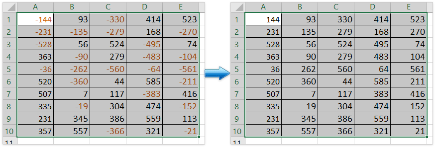
1. Rhowch rif -1 mewn cell wag, yna dewiswch y gell hon, a gwasgwch Ctrl + C allweddi i'w gopïo.
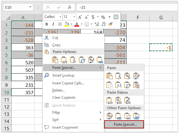
2. Dewiswch yr holl rifau negyddol yn yr ystod, cliciwch ar y dde, a dewiswch Gludo Arbennig ... o'r ddewislen cyd-destun. Gweler y screenshot:
(1) Daliad Ctrl allwedd, gallwch ddewis pob rhif negyddol trwy eu clicio fesul un;
(2) Os oes gennych chi Kutools ar gyfer Excel wedi'i osod, gallwch chi gymhwyso ei Dewiswch Gelloedd Arbennig nodwedd i ddewis yr holl rifau negyddol yn gyflym. Cael Treial Am Ddim!
3. Ac a Gludo arbennig bydd blwch deialog yn cael ei arddangos, dewiswch Popeth opsiwn o Gludo, dewiswch Lluoswch opsiwn o Ymgyrch, Cliciwch OK. Gweler y screenshot:

4. Bydd yr holl rifau negyddol a ddewisir yn cael eu trosi'n rhifau positif. Dileu'r rhif -1 yn ôl yr angen. Gweler y screenshot:

Newid rhifau negyddol yn hawdd i rai positif yn yr ystod benodol yn Excel
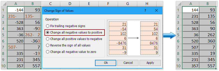
O'i gymharu â chael gwared ar yr arwydd negyddol o gelloedd un wrth un â llaw, Kutools ar gyfer Excel's Newid Arwydd Gwerthoedd nodwedd yn darparu ffordd hynod o hawdd i newid pob rhif negyddol yn gyflym i gadarnhaol wrth ddewis. Sicrhewch dreial 30 diwrnod llawn sylw am ddim nawr!
Kutools ar gyfer Excel - Supercharge Excel gyda dros 300 o offer hanfodol. Mwynhewch dreial 30 diwrnod llawn sylw AM DDIM heb fod angen cerdyn credyd! Get It Now
Yn gyflym ac yn hawdd newid rhifau negyddol i bositif gyda Kutools ar gyfer Excel
Nid yw'r mwyafrif o ddefnyddwyr Excel eisiau defnyddio cod VBA, a oes unrhyw driciau cyflym ar gyfer newid y rhifau negyddol yn bositif? Kutools ar gyfer excel yn gallu'ch helpu chi yn hawdd ac yn gyffyrddus i gyflawni hyn.
Kutools ar gyfer Excel - Supercharge Excel gyda dros 300 o offer hanfodol. Mwynhewch dreial 30 diwrnod llawn sylw AM DDIM heb fod angen cerdyn credyd! Get It Now
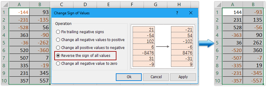
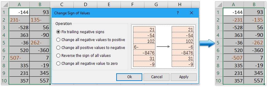
1. Dewiswch ystod gan gynnwys y rhifau negyddol rydych chi am eu newid, a chlicio Kutools > Cynnwys > Newid Arwydd Gwerthoedd.
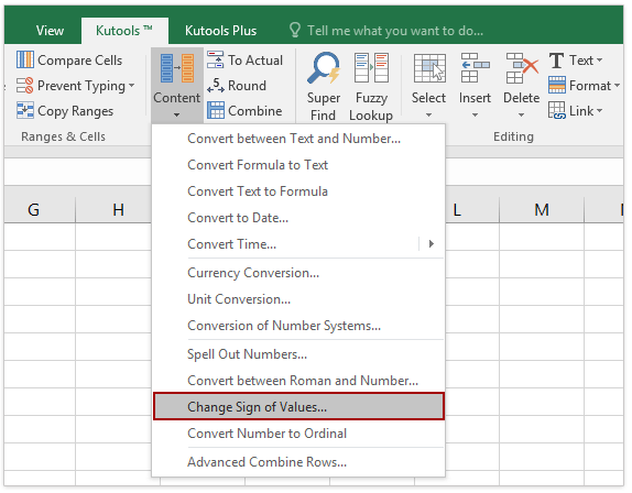
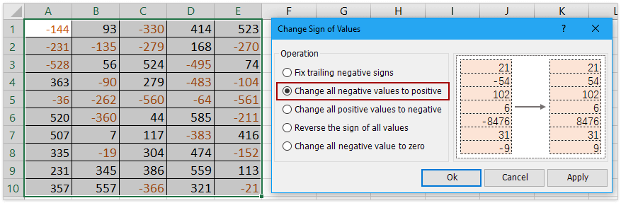
2. Gwirio Newid pob gwerth negyddol i bositif dan Ymgyrch, a chliciwch Ok. Gweler y screenshot:
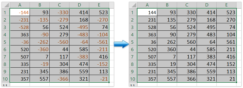
Nawr fe welwch yr holl rifau negyddol yn newid i rifau positif fel y dangosir isod:
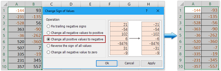
Nodyn: Gyda hyn Newid arwydd Gwerthoedd nodwedd, gallwch hefyd drwsio arwyddion negyddol sy'n llusgo, newid pob rhif positif i negyddol, gwrthdroi arwydd yr holl werthoedd a newid yr holl werthoedd negyddol i sero. Cael Treial Am Ddim!
(1) Newid yr holl werthoedd positif yn gyflym i negyddol yn yr ystod benodol:
(2) Gwrthdroi arwydd yr holl werthoedd yn yr ystod benodol yn hawdd:
(3) Newid yr holl werthoedd negyddol yn hawdd i sero yn yr ystod benodol:

(4) Trwsio arwyddion negyddol sy'n llusgo yn yr ystod benodol yn hawdd:
Defnyddio cod VBA i drosi holl rifau negyddol amrediad yn bositif
Fel gweithiwr proffesiynol Excel, gallwch hefyd redeg y cod VBA i newid y rhifau negyddol i rifau positif.
1. Pwyswch allweddi Alt + F11 i agor ffenestr Microsoft Visual Basic for Applications.
2. Bydd ffenestr newydd yn cael ei harddangos. Cliciwch Mewnosod > Modiwlau, yna mewnbwn y codau canlynol yn y modiwl:
Sub Positive
Dim Cel As Range
For Each Cel In Selection
If IsNumeric(Cel.Value) Then
Cel.Value = Abs(Cel.Value)
End If
Next Cel
End Sub3. Yna cliciwch Run botwm neu wasg F5 yn allweddol i redeg y cais, a bydd yr holl rifau negyddol yn cael eu newid i rifau positif. Gweler y screenshot:
Demo: Newid rhifau negyddol i bositif neu i'r gwrthwyneb gyda Kutools ar gyfer Excel
Erthyglau perthnasol
Gwrthdroi arwyddion gwerthoedd mewn celloedd
Pan ddefnyddiwn excel, mae rhifau cadarnhaol a negyddol mewn taflen waith. Gan dybio bod angen i ni newid y rhifau positif i rai negyddol ac i'r gwrthwyneb. Wrth gwrs, gallwn eu newid â llaw, ond os oes cannoedd o rifau mae angen eu newid, nid yw'r dull hwn yn ddewis da. A oes unrhyw driciau cyflym i ddatrys y broblem hon?
Newid rhifau positif i negyddol
Sut allwch chi newid yr holl rifau neu werthoedd positif i negyddol yn Excel? Gall y dulliau canlynol eich arwain i newid pob rhif positif i negyddol yn Excel yn gyflym.
Trwsiwch arwyddion negyddol sy'n llusgo mewn celloedd
Am rai rhesymau, efallai y bydd angen i chi drwsio arwyddion negyddol sy'n llusgo mewn celloedd yn Excel. Er enghraifft, byddai nifer ag arwyddion negyddol llusgo fel 90-. Yn y cyflwr hwn, sut allwch chi drwsio'r arwyddion negyddol sy'n llusgo'n gyflym trwy dynnu'r arwydd negyddol sy'n llusgo o'r dde i'r chwith? Dyma rai triciau cyflym a all eich helpu.
Newid rhif negyddol i sero
Byddaf yn eich arwain i newid pob rhif negyddol i sero ar unwaith yn y detholiad.
Yr Offer Cynhyrchedd Swyddfa Gorau
Kutools for Excel - Yn Eich Helpu i Sefyll Allan O Dyrfa
Kutools ar gyfer Excel Mae ganddo Dros 300 o Nodweddion, Sicrhau mai dim ond clic i ffwrdd yw'r hyn sydd ei angen arnoch chi...
")
Tab Office - Galluogi Darllen a Golygu Tabiau yn Microsoft Office (gan gynnwys Excel)
- Un eiliad i newid rhwng dwsinau o ddogfennau agored!
- Gostyngwch gannoedd o gliciau llygoden i chi bob dydd, ffarweliwch â llaw llygoden.
- Yn cynyddu eich cynhyrchiant 50% wrth wylio a golygu sawl dogfen.
- Yn dod â Thabiau Effeithlon i'r Swyddfa (gan gynnwys Excel), Just Like Chrome, Edge a Firefox.
")