Sut i newid lliw cefndir neu ffont yn seiliedig ar werth celloedd yn Excel?
Pan fyddwch chi'n delio â data enfawr yn Excel, efallai yr hoffech chi ddewis rhywfaint o werth a'u hamlygu â chefndir penodol neu liw ffont. Mae'r erthygl hon yn sôn am sut i newid cefndir neu liw ffont yn seiliedig ar werthoedd celloedd yn Excel yn gyflym.
Dull 2: Newid cefndir neu liw ffont yn seiliedig ar werth celloedd yn statig gyda swyddogaeth Find
Dull 1: Newid cefndir neu liw ffont yn seiliedig ar werth celloedd yn ddeinamig gyda Fformatio Amodol
Mae adroddiadau Fformatio Amodol gall nodwedd eich helpu i dynnu sylw at y gwerthoedd sy'n fwy na x, llai nag y, neu rhwng x ac y.
Gan dybio bod gennych chi ystod o ddata, a nawr bod angen i chi liwio'r gwerthoedd rhwng 80 a 100, gwnewch y camau canlynol:
1. Dewiswch yr ystod o gelloedd rydych chi am dynnu sylw at rai celloedd, ac yna cliciwch Hafan > Fformatio Amodol > Rheol Newydd, gweler y screenshot:

2. Yn y Rheol Fformatio Newydd blwch deialog, dewiswch y Fformatiwch gelloedd yn unig sy'n cynnwys eitem yn y Dewiswch Math o Reol blwch, ac yn y Fformat Celloedd yn Unig gyda adran, nodwch yr amodau sydd eu hangen arnoch:
- Yn y blwch gwympo cyntaf, dewiswch y Gwerth Cell;
- Yn yr ail flwch gwympo, dewiswch y meini prawf:rhwng;
- Yn y trydydd a'r pedwerydd blwch, nodwch yr amodau hidlo, fel 80, 100.

3. Yna, cliciwch fformat botwm, yn y Celloedd Fformat blwch deialog, gosodwch y cefndir neu'r lliw ffont fel hyn:
| Newidiwch y lliw cefndir yn ôl gwerth y gell: | Newid lliw'r ffont yn ôl gwerth y gell |
| Cliciwch Llenwch tab, ac yna dewiswch un lliw cefndir rydych chi'n ei hoffi | Cliciwch Ffont tab, a dewiswch y lliw ffont sydd ei angen arnoch chi. |
 |
 |
4. Ar ôl dewis y cefndir neu liw'r ffont, cliciwch OK > OK i gau'r dialogau, ac yn awr, mae'r celloedd penodol sydd â gwerth rhwng 80 a 100 yn cael eu newid i'r rhai penodol y cefndir neu'r lliw ffont yn y dewis. Gweler y screenshot:
| Tynnwch sylw at gelloedd penodol gyda lliw cefndir: | Tynnwch sylw at gelloedd penodol gyda lliw ffont: |
 |
 |
Nodyn: Y Fformatio Amodol yn nodwedd ddeinamig, bydd lliw'r gell yn cael ei newid wrth i'r data newid.
Dull 2: Newid cefndir neu liw ffont yn seiliedig ar werth celloedd yn statig gyda swyddogaeth Find
Weithiau, mae angen i chi gymhwyso lliw llenwi neu ffont penodol yn seiliedig ar werth y gell a gwneud i'r lliw llenwi neu ffont beidio â newid pan fydd gwerth y gell yn newid. Yn yr achos hwn, gallwch ddefnyddio'r Dod o hyd i swyddogaeth i ddod o hyd i'r holl werthoedd celloedd penodol ac yna newid cefndir neu liw ffont i'ch angen.
Er enghraifft, rydych chi am newid cefndir neu liw ffont os yw gwerth y gell yn cynnwys testun “Excel”, gwnewch fel hyn:
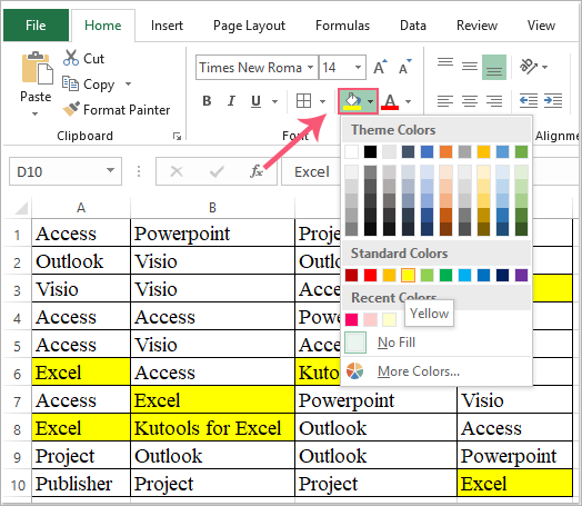
1. Dewiswch yr ystod ddata rydych chi am ei defnyddio, ac yna cliciwch Hafan > Dod o Hyd i a Dewis > Dod o hyd i, gweler y screenshot:

2. Yn y Dod o hyd ac yn ei le blwch deialog, o dan y Dod o hyd i tab, nodwch y gwerth rydych chi am ei ddarganfod yn y Dewch o hyd i beth blwch testun, gweler y screenshot:

3. Ac yna, cliciwch Dewch o Hyd i Bawb botwm, yn y blwch darganfod canlyniadau, cliciwch unrhyw un eitem, ac yna pwyswch Ctrl + A i ddewis yr holl eitemau a ddarganfuwyd, gweler y screenshot:

4. O'r diwedd, cliciwch Cau botwm i gau'r ymgom hwn. Nawr, gallwch chi lenwi cefndir neu liw ffont ar gyfer y gwerthoedd dethol hyn, gweler y screenshot:
| Defnyddiwch y lliw cefndir ar gyfer y celloedd a ddewiswyd: | Defnyddiwch liw'r ffont ar gyfer y celloedd a ddewiswyd: |
 |
 |
Dull 3: Newid lliw cefndir neu ffont yn seiliedig ar werth celloedd yn statig gyda Kutools ar gyfer Excel
Kutools ar gyfer Excel'S Super Darganfod nodwedd yn cefnogi llawer o amodau ar gyfer dod o hyd i werthoedd, llinynnau testun, dyddiadau, fformwlâu, celloedd wedi'u fformatio ac ati. Ar ôl dod o hyd i'r celloedd sydd wedi'u paru a'u dewis, gallwch chi newid y cefndir neu'r lliw ffont i'r hyn rydych chi ei eisiau.
Ar ôl gosod Kutools ar gyfer Excel, gwnewch fel hyn:
1. Dewiswch yr ystod ddata rydych chi am ddod o hyd iddi, ac yna cliciwch Kutools > Super Darganfod, gweler y screenshot:

2. Yn y Super Darganfod cwarel, gwnewch y gweithrediadau canlynol:
- (1.) Yn gyntaf, cliciwch y Gwerthoedd eicon opsiwn;
- (2.) Dewiswch y cwmpas darganfod o'r Yn gollwng, yn yr achos hwn, byddaf yn dewis Dewis;
- (3.) O'r math rhestr ostwng, dewiswch y meini prawf rydych chi am eu defnyddio;
- (4.) Yna cliciwch Dod o hyd i botwm i restru'r holl ganlyniadau cyfatebol yn y blwch rhestr;
- (5.) O'r diwedd, cliciwch dewiswch botwm i ddewis y celloedd.

3. Ac yna, mae'r holl gelloedd sy'n cyfateb i'r meini prawf wedi'u dewis ar unwaith, gweler y screenshot:

4. Ac yn awr, gallwch newid y lliw cefndir neu'r lliw ffont ar gyfer y celloedd a ddewiswyd yn ôl yr angen.
Awgrymiadau: Efo'r Super Darganfod swyddogaeth, gallwch hefyd ddelio â'r gweithrediadau canlynol yn gyflym ac yn hawdd:
Gwaith prysur ar benwythnos, Defnyddiwch Kutools ar gyfer Excel,
yn rhoi penwythnos hamddenol a llawen i chi!
Ar y penwythnos, mae'r plant yn glampio i fynd allan i chwarae, ond mae gormod o waith yn eich amgylchynu i gael amser i fynd gyda'r teulu. Yr haul, y traeth a'r môr mor bell i ffwrdd? Kutools ar gyfer Excel yn eich helpu i datrys posau Excel, arbed amser gwaith.

- Nid yw cael dyrchafiad a chynyddu cyflog yn bell;
- Yn cynnwys nodweddion uwch, datrys senarios cais, mae rhai nodweddion hyd yn oed yn arbed 99% o amser gwaith;
- Dewch yn arbenigwr Excel mewn 3 munud, a chael cydnabyddiaeth gan eich cydweithwyr neu ffrindiau;
- Nid oes angen chwilio atebion gan Google mwyach, ffarwelio â fformwlâu poenus a chodau VBA;
- Gellir cwblhau'r holl lawdriniaethau dro ar ôl tro gyda dim ond sawl clic, rhyddhewch eich dwylo blinedig;
- Dim ond $ 39 ond yn werth na thiwtorial Excel $ 4000 y bobl eraill;
- Cael eich dewis gan 110,000 o elites a 300+ o gwmnïau adnabyddus;
- Treial am ddim 30 diwrnod, ac arian llawn yn ôl o fewn 60 diwrnod heb unrhyw reswm;
- Newidiwch y ffordd rydych chi'n gweithio, ac yna newid eich ffordd o fyw!