Skip i'r prif gynnwys

Sut i ddod o hyd i'r nawfed gell nad yw'n wag yn Excel?

Sut allech chi ddod o hyd i'r nawfed gwerth celloedd nad yw'n wag o golofn neu res yn Excel? Yr erthygl hon, byddaf yn siarad am rai fformiwlâu defnyddiol i chi ddatrys y dasg hon.

Darganfyddwch a dychwelwch y nawfed gwerth celloedd nad yw'n wag o golofn â fformiwla

Darganfyddwch a dychwelwch y nawfed gwerth celloedd nad yw'n wag o res gyda fformiwla


swigen dde glas saeth Darganfyddwch a dychwelwch y nawfed gwerth celloedd nad yw'n wag o golofn â fformiwla

Er enghraifft, mae gen i golofn o ddata fel y dangosir ar-lein, nawr, byddaf yn cael y trydydd gwerth celloedd nad yw'n wag o'r rhestr hon.

doc dod o hyd i nth yn wag 1

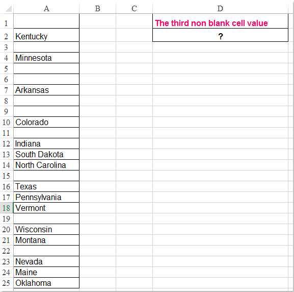
Rhowch y fformiwla hon: =INDEX($A$1:$A$25,SMALL(ROW($A$1:$A$25)+(100*($A$1:$A$25="")), 3))&"" i mewn i gell wag lle rydych chi am allbwn y canlyniad, D2, er enghraifft, ac yna pwyswch Ctrl + Shift + Enter allweddi gyda'i gilydd i gael y canlyniad cywir, gweler y screenshot:

doc dod o hyd i nth yn wag 2

Nodyn: Yn y fformiwla uchod, A1: A25 yw'r rhestr ddata rydych chi am ei defnyddio, a'r rhif 3 yn nodi'r trydydd gwerth cell nad yw'n wag yr ydych am ei ddychwelyd, os ydych am gael yr ail gell nad yw'n wag, dim ond newid y rhif 3 i 2 sydd ei angen arnoch.


swigen dde glas saeth Darganfyddwch a dychwelwch y nawfed gwerth celloedd nad yw'n wag o res gyda fformiwla

Os ydych chi am ddarganfod a dychwelyd y nawfed gwerth celloedd nad yw'n wag yn olynol, gall y fformiwla ganlynol eich helpu chi, gwnewch fel hyn:

Rhowch y fformiwla hon: =INDEX($A$1:$M$1,SMALL(IF($A$1:$M$1<>"",COLUMN($A$1:$M$1)-COLUMN($A$1)+1),4)) i mewn i gell wag lle rydych chi am ddod o hyd i'r canlyniad, ac yna pwyso Ctrl + Shift + Enter allweddi gyda'i gilydd i gael y canlyniad, gweler y screenshot:

doc dod o hyd i nth yn wag 3

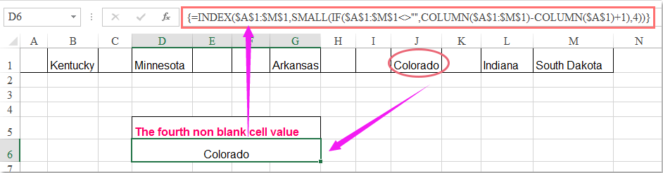
Nodyn: Yn y fformiwla uchod, A1: M1 yw'r gwerthoedd rhes rydych chi am eu defnyddio, a'r rhif 4 yw'r pedwerydd gwerth cell nad yw'n wag yr ydych am ei ddychwelyd, os ydych chi am gael yr ail gell nad yw'n wag, mae angen ichi newid y rhif 4 i 2 yn ôl yr angen.

Offer Cynhyrchiant Swyddfa Gorau

🤖 Kutools AI Aide: Chwyldro dadansoddi data yn seiliedig ar: Cyflawniad Deallus   |  Cynhyrchu Cod  |  Creu Fformiwlâu Personol  |  Dadansoddi Data a Chynhyrchu Siartiau  |  Invoke Swyddogaethau Kutools...
Nodweddion Poblogaidd: Darganfod, Amlygu neu Adnabod Dyblygiadau   |  Dileu Rhesi Gwag   |  Cyfuno Colofnau neu Gelloedd heb Colli Data   |   Rownd heb Fformiwla ...
Super-edrych: VLookup Meini Prawf Lluosog    VLookup Gwerth Lluosog  |   VLookup Ar Draws Taflenni Lluosog   |   Edrych Niwlog ....
Rhestr gwympo Uwch: Creu Rhestr Gollwng yn Gyflym   |  Rhestr Gollwng Dibynnol   |  Rhestr Gollwng Aml-ddewis ....
Rheolwr Colofn: Ychwanegu Nifer Penodol o Golofnau  |  Symud Colofnau  |  Toglo Statws Gwelededd Colofnau Cudd  |  Cymharwch Ystodau a Cholofnau ...
Nodweddion dan Sylw: Ffocws ar y Grid   |  Golwg Dylunio   |   Bar Fformiwla Mawr    Rheolwr Llyfr Gwaith a Thaflen   |  Llyfrgell Adnoddau (Testun Auto)   |  Dewiswr Dyddiad   |  Cyfuno Taflenni Gwaith   |  Amgryptio/Dadgryptio Celloedd    Anfon E-byst trwy Restr   |  Hidlo Super   |   Hidlo Arbennig (hidlo mewn print trwm/italig/strikethrough...) ...
15 Set Offer Gorau12 Testun offer (Ychwanegu Testun, Dileu Cymeriadau,...)   |   50 + Siart Mathau (Siart Gantt,...)   |   40+ Ymarferol Fformiwlâu (Cyfrifwch oedran yn seiliedig ar ben-blwydd,...)   |   19 mewnosod offer (Mewnosod Cod QR, Mewnosod Llun o'r Llwybr,...)   |   12 Trosi offer (Rhifau i Eiriau, Trosi arian cyfred,...)   |   7 Uno a Hollti offer (Rhesi Cyfuno Uwch, Celloedd Hollt,...)   |   ... a mwy

Supercharge Eich Sgiliau Excel gyda Kutools ar gyfer Excel, a Phrofiad Effeithlonrwydd Fel Erioed Erioed. Kutools ar gyfer Excel Yn Cynnig Dros 300 o Nodweddion Uwch i Hybu Cynhyrchiant ac Arbed Amser.  Cliciwch Yma i Gael Y Nodwedd Sydd Ei Angen Y Mwyaf...

Disgrifiad


Mae Office Tab yn dod â rhyngwyneb Tabbed i Office, ac yn Gwneud Eich Gwaith yn Haws o lawer

  • Galluogi golygu a darllen tabbed yn Word, Excel, PowerPoint, Cyhoeddwr, Mynediad, Visio a Phrosiect.
  • Agor a chreu dogfennau lluosog mewn tabiau newydd o'r un ffenestr, yn hytrach nag mewn ffenestri newydd.
  • Yn cynyddu eich cynhyrchiant 50%, ac yn lleihau cannoedd o gliciau llygoden i chi bob dydd!
Comments (10)
No ratings yet. Be the first to rate!
This comment was minimized by the moderator on the site
CIAO STO CERCANDO DI APPLICARE LA TUA FORMULA MA NON MI FUNZIONA, DOVE STO SBAGLIANDO?
=INDICE($K$37:$K$88;MIN(RIGHE($K$37:$K$88)+RIGHE(100*($K$37:$K$88=""));6))&""
DEVO VISUALIZZARE L'ENNESIMA RIGA DIVERSA DA VUOTO

GRAzie
This comment was minimized by the moderator on the site
=INDICE($K$37:$K$88;MIN(RIGHE($K$37:$K$88)+(100*($K$37:$K$88=""));6))&""
This comment was minimized by the moderator on the site
I'm running this formula on a ~400 row sheet with around 20 blanks mixed throughout the data, and it's working perfectly EXCEPT when I fill the series down, it sometimes duplicates a row for some reason. For example, it seems to think a value is somehow simultaneously the 331st non-blank and the 332nd.

Things I've noticed:
-Duplications always happen in pairs (ex. 331 and 332 are duplicates, 333 and 334 will also be), then it goes back to normal for a while.
-Raw data also has blanks in pairs, but not corresponding to the duplicates
-No duplications occur in the first 94 rows, but they happen every 33-35 rows after that
-Does not appear to be linked to the value in the cell being duplicated
-I have entered as an array and as a standard formula, no difference in function

For reference, here's my actual formula:

=INDEX('PO Raw Data'!CR:CR,SMALL(ROW('PO Raw Data'!CR:CR)+(100*('PO Raw Data'!CR:CR="")),$W2)&"")

Note $W2 refers to a helper column and counts up as the data set is filled down, but only because I couldn't get it to count up when I just used a number instead of cell reference.
When I've replaced that cell reference (ex. $W2) with the appropriate number, same result.


Any thoughts on what I can do to fix that?
This comment was minimized by the moderator on the site
very helpful,
although when I return the nth non blank cell in a column set to DATE, the returned value appears as number(general number).formatting the cell into DATE also doesn't change the result. could you please give me a hand!
thanks a lot
This comment was minimized by the moderator on the site
Hello, Shirazi,
Sorry, maybe there is no direct formula for you to get the date format.

If someone else has the solution, please comment here.
This comment was minimized by the moderator on the site
Hi everyone!


Could you also help me return the row number of the second, third non-blank cell?


Please help me.
This comment was minimized by the moderator on the site
Hello, John,
the following formula can help you to get all the row numbers of the non-blank cells, please try it, thank you!
=IFERROR(ROW(INDEX($A$1:$A$12,SMALL(INDEX(NOT(ISBLANK($A$1:$A$12))*ROW($A$1:$A$12),0),COUNTBLANK($A$1:$A$12)+ROW(A1)))),"")
This comment was minimized by the moderator on the site
Hey everyone,

I have a table with numerous columns and rows. The rows have range names, and a description/location at the beginning of the row range with its own range, example "Building No.s". There are multiple Row Ranges/ Buildings. There are headers at the top of each columns for specific "Building Assembly Types". The table content is numeric quantities for each type "Building Assembly Type" for each specific "Building" description/location. There could be as many as (100) "Building Assembly Types" column headers but I will limit the assemblies to (10) per row range, so there will be numerous blank cells in each "Building No." range.

I have other summary tables set up for each "Building" that I want to pull the non-blank cells quantities to, along with the corresponding header "Assembly Type" for each "Building" with a (10) max "Assemblies" per page.

I can identify the non-blank cell quantities by use of the array formula above for rows. The problem I am having is identifying the header that corresponds to it.

Ultimately if I can identify the "Assembly" header, I can always index the "Quantities" once I have the header "Assembly" identified for each "Building". Then I would be able do a lookup for all the parts associated with each "Assembly" type for that "Building" from my Assembly parts database and multiply it times the "Quantity" of each assembly type.

Hopefully this makes since and someone can help.
This comment was minimized by the moderator on the site
Hello, I am looking for the third blank row in a column and I copied your formula and just changed the range from $A$1:$A:$25 to my range $D$306:$D$354. But when I change the range I get #REF! as my answer. I already converted to an array, control-shift-enter. Now the cell range I am referencing has formulas in them, so could that be why I am getting #REF. Your formula: =INDEX($A$1:$A$25,SMALL(ROW($A$1:$A$25)+(100*($A$1:$A$25="")), 3))&"" My formula: =INDEX($D$306:$D$354,SMALL(ROW($D$306:$D$354)+(1*($D$306:$D$354="")), 2))&"" Thanks, Noel
This comment was minimized by the moderator on the site
you have put the 1 instead of 100 therefore answered was wrong. please use below formula

INDEX($D$306:$D$354,SMALL(ROW($D$306:$D$354)+(100*($D$306:$D$354="")), 3))&"" than ctrl + shift+enter
There are no comments posted here yet
Please leave your comments in English
Posting as Guest
×
Rate this post:
0   Characters
Suggested Locations