Skip i'r prif gynnwys

Sut i ddiffinio ystod yn seiliedig ar werth cell arall yn Excel?

Mae cyfrifo ystod o werthoedd yn hawdd i'r mwyafrif o ddefnyddwyr Excel, ond a ydych erioed wedi ceisio cyfrifo ystod o werthoedd yn seiliedig ar y nifer mewn cell benodol? Er enghraifft, mae colofn o werthoedd yng ngholofn A, ac rwyf am gyfrifo nifer y gwerthoedd yng ngholofn A yn seiliedig ar y gwerth yn B2, sy'n golygu, os yw'n 4 yn B2, y byddaf yn cyfartaleddu'r 4 gwerth cyntaf yn colofn A fel y dangosir isod. Nawr rwy'n cyflwyno fformiwla syml i ddiffinio ystod yn gyflym yn seiliedig ar werth cell arall yn Excel.
doc diffinio ystod yn ôl gwerth cell 1

Diffinio ystod yn seiliedig ar werth celloedd


swigen dde glas saeth Diffinio ystod yn seiliedig ar werth celloedd

I gyfrifo am ystod yn seiliedig ar werth cell arall, gallwch ddefnyddio fformiwla syml.

Dewiswch gell wag y byddwch chi'n ei rhoi allan o'r canlyniad, nodwch y fformiwla hon = CYFARTAL (A1: INDIRECT (CONCATENATE ("A", B2))), a'r wasg Rhowch allwedd i gael y canlyniad.
doc diffinio ystod yn ôl gwerth cell 2

Nodyn:

1. Yn y fformiwla, A1 yw'r gell gyntaf yn y golofn rydych chi am ei chyfrifo, A yw'r golofn rydych chi'n cyfrif amdani, B2 yw'r gell rydych chi'n ei chyfrifo yn seiliedig arni. Gallwch chi newid y cyfeiriadau hyn yn ôl yr angen.

2. Os ydych chi am wneud crynodeb, gallwch ddefnyddio'r fformiwla hon = SUM (A1: INDIRECT (CONCATENATE ("A", B2))).

3. Os nad yw'r data cyntaf yr ydych am ei ddiffinio yn rhes gyntaf yn yr Excel, er enghraifft, yng nghell A2, gallwch ddefnyddio'r fformiwla fel hyn: = CYFARTAL (A2: INDIRECT (CONCATENATE ("A", ROW (A2) + B2-1))).
doc diffinio ystod yn ôl gwerth cell 2


Cyfrif / Swmio celloedd yn gyflym yn ôl cefndir neu liw fformat yn Excel

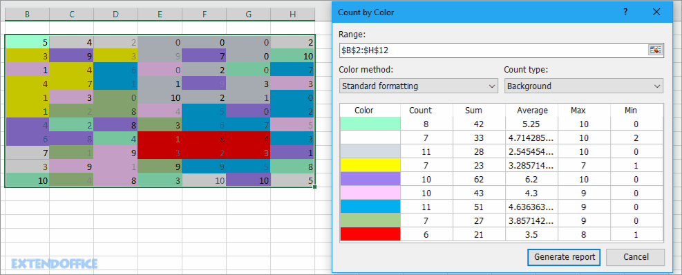
Mewn rhai achosion, efallai bod gennych chi ystod o gelloedd â lliwiau lluosog, a'r hyn rydych chi ei eisiau yw cyfrif / swm gwerthoedd yn seiliedig ar yr un lliw, sut allwch chi gyfrifo'n gyflym?
Gyda Kutools ar gyfer Excel's Cyfrif yn ôl Lliw, gallwch chi wneud llawer o gyfrifiadau yn gyflym yn ôl lliw, a hefyd gallwch gynhyrchu adroddiad o'r canlyniad a gyfrifwyd.  Cliciwch i gael treial llawn am ddim mewn 30 diwrnod!
cyfrif doc yn ôl lliw 1
 
Kutools ar gyfer Excel: gyda mwy na 300 o ychwanegion Excel defnyddiol, am ddim i geisio heb unrhyw gyfyngiad mewn 30 diwrnod.

Offer Cynhyrchiant Swyddfa Gorau

🤖 Kutools AI Aide: Chwyldro dadansoddi data yn seiliedig ar: Cyflawniad Deallus   |  Cynhyrchu Cod  |  Creu Fformiwlâu Personol  |  Dadansoddi Data a Chynhyrchu Siartiau  |  Invoke Swyddogaethau Kutools...
Nodweddion Poblogaidd: Darganfod, Amlygu neu Adnabod Dyblygiadau   |  Dileu Rhesi Gwag   |  Cyfuno Colofnau neu Gelloedd heb Colli Data   |   Rownd heb Fformiwla ...
Super-edrych: VLookup Meini Prawf Lluosog    VLookup Gwerth Lluosog  |   VLookup Ar Draws Taflenni Lluosog   |   Edrych Niwlog ....
Rhestr gwympo Uwch: Creu Rhestr Gollwng yn Gyflym   |  Rhestr Gollwng Dibynnol   |  Rhestr Gollwng Aml-ddewis ....
Rheolwr Colofn: Ychwanegu Nifer Penodol o Golofnau  |  Symud Colofnau  |  Toglo Statws Gwelededd Colofnau Cudd  |  Cymharwch Ystodau a Cholofnau ...
Nodweddion dan Sylw: Ffocws ar y Grid   |  Golwg Dylunio   |   Bar Fformiwla Mawr    Rheolwr Llyfr Gwaith a Thaflen   |  Llyfrgell Adnoddau (Testun Auto)   |  Dewiswr Dyddiad   |  Cyfuno Taflenni Gwaith   |  Amgryptio/Dadgryptio Celloedd    Anfon E-byst trwy Restr   |  Hidlo Super   |   Hidlo Arbennig (hidlo mewn print trwm/italig/strikethrough...) ...
15 Set Offer Gorau12 Testun offer (Ychwanegu Testun, Dileu Cymeriadau,...)   |   50 + Siart Mathau (Siart Gantt,...)   |   40+ Ymarferol Fformiwlâu (Cyfrifwch oedran yn seiliedig ar ben-blwydd,...)   |   19 mewnosod offer (Mewnosod Cod QR, Mewnosod Llun o'r Llwybr,...)   |   12 Trosi offer (Rhifau i Eiriau, Trosi arian cyfred,...)   |   7 Uno a Hollti offer (Rhesi Cyfuno Uwch, Celloedd Hollt,...)   |   ... a mwy

Supercharge Eich Sgiliau Excel gyda Kutools ar gyfer Excel, a Phrofiad Effeithlonrwydd Fel Erioed Erioed. Kutools ar gyfer Excel Yn Cynnig Dros 300 o Nodweddion Uwch i Hybu Cynhyrchiant ac Arbed Amser.  Cliciwch Yma i Gael Y Nodwedd Sydd Ei Angen Y Mwyaf...

Disgrifiad


Mae Office Tab yn dod â rhyngwyneb Tabbed i Office, ac yn Gwneud Eich Gwaith yn Haws o lawer

  • Galluogi golygu a darllen tabbed yn Word, Excel, PowerPoint, Cyhoeddwr, Mynediad, Visio a Phrosiect.
  • Agor a chreu dogfennau lluosog mewn tabiau newydd o'r un ffenestr, yn hytrach nag mewn ffenestri newydd.
  • Yn cynyddu eich cynhyrchiant 50%, ac yn lleihau cannoedd o gliciau llygoden i chi bob dydd!
Comments (21)
No ratings yet. Be the first to rate!
This comment was minimized by the moderator on the site
But If I want to sum a column range(say l7:l7800) out of the range d7:ct9000 based on the condition in column a(a7:a9000) and column b(b7:b9000). How will I do it. Please advise
This comment was minimized by the moderator on the site
Is there a way to create a dynamic ranged view, that will isolate all orders from a specific client within a list of clients? I have looked at multiple videos and none actually do what I need it to do. Is there a way to do this or would I need to pull the needed info into a controlled table and use the information from that table?
This comment was minimized by the moderator on the site
Hi, CareTaker. I do not get your question clearly. Could you describe your question or upload a file to show the quetion in details? But I recomend a utility called Data Association for you, maybe can help you, go to this web for details: https://www.extendoffice.com/product/kutools-for-excel/excel-click-cell-to-filter-based-on-another-workbook.html.
This comment was minimized by the moderator on the site
Thank you for the response, its quite the complicated thing to explain but I did manage to come right in the end using the indexing formula with the match formula as well.   =INDEX($B:$B;MATCH($C$2;$B:$B;0);):INDEX($N:$N;MATCH($C$2;$B:$B;0)+$C$3-1;)   at first it was confusing but I'm good now 
This comment was minimized by the moderator on the site
how do I update sum range by using helper cell...For example: if initial sum range is = C1 to M1, how to do change sum range if new data is up to AB1 using a helper cell, instead of changing the formula manually?
This comment was minimized by the moderator on the site
What if the rage is not column, but a row?
This comment was minimized by the moderator on the site
That's a bit trickier as I just found out. You need to use a combination of the CHAR function to convert a number to a letter, CONCAT to piece together a letter and number comprising a cell address, and the INDIRECT function to recognize strings as cell addresses.

In my example, I wrote the following expression:

=SUM(INDIRECT(CONCAT("F",ROW())):INDIRECT(CONCAT(CHAR(64+5+$B$31),ROW())))


where:
Row() is the current row
$B$31 is the cell where the # of columns to count is stored
5 is the offset for the first column to be counted

if you need to go beyond column Z, you’d need a less intuitive variant on that expression using the ADDRESS function:

=SUM(indirect(concat("F",row())):indirect(ADDRESS(row(),$B$31+5,4)))


where:
4 indicates a relative reference
This comment was minimized by the moderator on the site
Hi quick question. My formula =SUMIFS(DATA!$D$5:$D$13914,DATA!$E$5:INDIRECT(CONCATENATE("$E$",C3)),"<"&"1/1/2016") has a range that is from another tab called "DATA." I keep getting #VALUE! errors for this formula. Any suggestions? thanks!
This comment was minimized by the moderator on the site
Earlier I posted: Great formula but why does it only work when referring to the first cell. In other words, if you move the whole range down and the first cell in the range is A5 instead of A1, the formula ceases to work.
After playing with it, I figured out why the formula is not working when the starting row is not row 1. Excel interprets this as the range being A1 thru A4. If you are starting with a different row than row 1, here is how to modify the formula assuming the range now starts with A5:=MAX(A5:INDIRECT(CONCATENATE("A",ROW(A5)+B2)))
This works because the concatenation sees the row reference as fixed in the first example, but it becomes relative in the second example. Hope that helps!
Jared - You can just subtract 4 instead of adding. =MAX(A5:INDIRECT(CONCATENATE("A",ROW(A5)-B2))) [Assuming you have 4 in cell B2, or you could just leave the formula as is and put -4 in cell B2.]
This comment was minimized by the moderator on the site
Hi,cathy, thanks for your supplement, I have test your formula, I think the correct formula may be =MAX(A5:INDIRECT(CONCATENATE("A",ROW(A5)+B2-1))). I have update the tutorual. Thanks again.
This comment was minimized by the moderator on the site
Great formula but why does it only work when referring to the first cell. In other words, if you move the whole range down and the first cell in the range is A6 instead of A1, the formula ceases to work. That seems strange.
This comment was minimized by the moderator on the site
What if I want to count upward from a cell rather than downward? In the above example, the formula starts with A1 and goes downward. Let's say I want a range of 4 cells, beginning with Cell A10 and going to A6. Thank you!
This comment was minimized by the moderator on the site
Jared - See my most recent post for how to solve this.
This comment was minimized by the moderator on the site
I'm having this upward problem also but unable to see your other post for the solution. Can you give me link of the post please? Many thanks!
This comment was minimized by the moderator on the site
Hi, here is a formula may help you to calcualte upward.
=AVERAGE(INDIRECT(CONCATENATE("A",COUNT(A:A)-B1+1)):INDIRECT(CONCATENATE("A",COUNT(A:A))))
A:A is the column that you want to calcualte the average values, B1 is the cell that define the range in column A to calculate.
This comment was minimized by the moderator on the site
Thanks, but may I know why need to use "-B1+1" please?
This comment was minimized by the moderator on the site
Hi, Let me take a detailed example to explain it for you. There are 10 rows in column A, I want to get the last 2 values' average, in other words, average the values in row 9 and row 10. Now B1 contains 2, =COUNT(A:A)-B1+1 will get the result 9, COUNT(A:A) will get the result 10 (the last row of the column A). Now combine other functions to averaget the values in row 9 and row 10. Hope this can help you.
This comment was minimized by the moderator on the site
Can I use this syntax while referring to a different sheet?
This comment was minimized by the moderator on the site
If you want to sum referring to a Different Shet In CONCATENATE formula write [ SHEET NAME+COLUMN+ROW]
Formula=SUM(INDIRECT(CONCATENATE("Sheet1!","D",1)):INDIRECT(CONCATENATE("Sheet1!","D",5)))
This comment was minimized by the moderator on the site
Hi, Thank you so much for your help, but I have a small problem that is I don't have just one column but several ones (about 100 columns) is there a way to change the formula to accommodate the change in columns so O can get the sum for Columns A B C and so on. thanks for your help
This comment was minimized by the moderator on the site
Thank u for your message. If you want to sum first n values across multiple continuous columns, just change A to the last column you ues. EG, sum first 5 values across column A to column D, apply this formula =SUM(A1:INDIRECT(CONCATENATE("D",F2))).
There are no comments posted here yet
Please leave your comments in English
Posting as Guest
×
Rate this post:
0   Characters
Suggested Locations