Sut i wyrdroi arwyddion gwerthoedd mewn celloedd yn Excel?
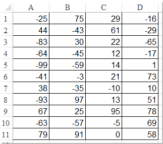
Pan ddefnyddiwn excel, mae rhifau cadarnhaol a negyddol mewn taflen waith. Gan dybio bod angen i ni newid y rhifau positif i rai negyddol ac i'r gwrthwyneb. Wrth gwrs, gallwn eu newid â llaw, ond os oes cannoedd o rifau mae angen eu newid, nid yw'r dull hwn yn ddewis da. A oes unrhyw driciau cyflym i ddatrys y broblem hon?
 |
 |
 |
Gwrthdroi'r arwydd o werthoedd mewn celloedd sydd â swyddogaeth Gludo Arbennig
Gwrthdroi'r arwydd o werthoedd mewn celloedd gyda Kutools ar gyfer Excel yn gyflym
Gwrthdroi'r arwydd o werthoedd mewn celloedd sydd â chod VBA
Gwrthdroi'r arwydd o werthoedd mewn celloedd sydd â swyddogaeth Gludo Arbennig

Gallwn wyrdroi'r arwydd o werthoedd mewn celloedd gyda'r Gludo Arbennig swyddogaeth yn Excel, gwnewch fel a ganlyn:
1. Rhif tap -1 mewn cell wag a'i chopïo.
2. Dewiswch yr ystod rydych chi am wyrdroi'r arwydd gwerthoedd, de-gliciwch a dewis Gludo Arbennig. Gweler y screenshot:

3. Yn y Gludo Arbennig blwch deialog, cliciwch Popeth opsiynau o Gludo ac Lluoswch opsiwn o Ymgyrch. Gweler y screenshot:

4. Yna cliciwch OK, ac mae holl arwyddion y rhifau yn yr ystod wedi'u gwrthdroi.
|
|
|
5. Dileu'r rhif -1 yn ôl yr angen.
Gwrthdroi arwydd yr holl rifau ar unwaith
Kutools ar gyfer Excel'S Newid Arwydd Gwerthoedd gall cyfleustodau eich helpu chi i newid y rhifau positif i negyddol ac i'r gwrthwyneb, gall hefyd eich helpu i wyrdroi arwydd y gwerthoedd a gosod arwydd negyddol sy'n llusgo i normal. Cliciwch i lawrlwytho Kutools ar gyfer Excel!

Kutools ar gyfer Excel: gyda mwy na 300 o ychwanegiadau Excel defnyddiol, am ddim i geisio heb unrhyw gyfyngiad mewn 30 diwrnod. Dadlwythwch a threial am ddim Nawr!
Gwrthdroi'r arwydd o werthoedd mewn celloedd gyda Kutools ar gyfer Excel yn gyflym
Gallwn wyrdroi'r arwydd o werthoedd yn gyflym gyda Newid Arwydd Gwerthoedd nodwedd o Kutools ar gyfer Excel.
| Kutools ar gyfer Excel : gyda mwy na 300 o ychwanegiadau Excel defnyddiol, am ddim i geisio heb unrhyw gyfyngiad mewn 30 diwrnod. |
Ar ôl gosod Kutools ar gyfer Excel, gwnewch fel a ganlyn:
1. Dewiswch yr ystod rydych chi am wyrdroi arwyddion y rhifau.
2. Cliciwch Kutools > Cynnwys > Newid Arwydd Gwerthoedd…, Gweler y screenshot:

3. Yn y Newid Arwydd Gwerthoedd blwch deialog, gwiriwch y Gwrthdroi arwydd yr holl werthoedd, gweler y screenshot:

4. Ac yna cliciwch OK or Gwneud cais. Mae holl arwyddion y rhifau wedi'u gwrthdroi.
- I ddefnyddio'r nodwedd hon, dylech osod Kutools ar gyfer Excel yn gyntaf, os gwelwch yn dda cliciwch i lawrlwytho a chael treial am ddim 30 diwrnod yn awr.
- Mae adroddiadau Newid Arwydd Gwerthoedd o Kutools ar gyfer Excel gall hefyd trwsio arwyddion negyddol sy'n llusgo, chongian yr holl werthoedd negyddol yn bositif ac newid yr holl werthoedd cadarnhaol i negyddol. Am wybodaeth fanylach am Newid Arwydd Gwerthoedd, Ewch i Newid disgrifiad nodwedd Sign of Values.
Gwrthdroi'r arwydd o werthoedd mewn celloedd sydd â chod VBA
Hefyd, gallwn ddefnyddio cod VBA i wyrdroi arwydd gwerthoedd mewn celloedd. Ond mae'n rhaid i ni wybod sut i gael y VBA i wneud y peth. Gallwn ei wneud fel y camau canlynol:
1. Dewiswch yr ystod rydych chi am wyrdroi'r arwydd gwerthoedd mewn celloedd.
2. Cliciwch Datblygwr > Visual Basic yn Excel, newydd Microsoft Visual Basic ar gyfer cymwysiadau bydd ffenestr yn cael ei harddangos, neu'n defnyddio'r bysellau llwybr byr (Alt + F11) i'w actifadu. Yna cliciwch Mewnosod > Modiwlau, ac yna copïwch a gludwch y cod VBA canlynol:
Sub Convert()
Dim C As Range
For Each C In Selection
C.Value = -C.Value
Next C
End Sub
3. Yna cliciwch ![]() botwm i redeg y cod. Ac mae'r arwydd o rifau yn yr ystod a ddewiswyd wedi'i wrthdroi ar unwaith.
botwm i redeg y cod. Ac mae'r arwydd o rifau yn yr ystod a ddewiswyd wedi'i wrthdroi ar unwaith.
Gwrthdroi'r arwydd o werthoedd mewn celloedd gyda Kutools ar gyfer Excel
Erthyglau perthnasol
Gwrthdroi arwyddion gwerthoedd mewn celloedd
Pan ddefnyddiwn excel, mae rhifau cadarnhaol a negyddol mewn taflen waith. Gan dybio bod angen i ni newid y rhifau positif i rai negyddol ac i'r gwrthwyneb. Wrth gwrs, gallwn eu newid â llaw, ond os oes cannoedd o rifau mae angen eu newid, nid yw'r dull hwn yn ddewis da. A oes unrhyw driciau cyflym i ddatrys y broblem hon?
Newid rhifau positif i negyddol
Sut allwch chi newid yr holl rifau neu werthoedd positif i negyddol yn Excel? Gall y dulliau canlynol eich arwain i newid pob rhif positif i negyddol yn Excel yn gyflym.
Trwsiwch arwyddion negyddol sy'n llusgo mewn celloedd
Am rai rhesymau, efallai y bydd angen i chi drwsio arwyddion negyddol sy'n llusgo mewn celloedd yn Excel. Er enghraifft, byddai nifer ag arwyddion negyddol llusgo fel 90-. Yn y cyflwr hwn, sut allwch chi drwsio'r arwyddion negyddol sy'n llusgo'n gyflym trwy dynnu'r arwydd negyddol sy'n llusgo o'r dde i'r chwith? Dyma rai triciau cyflym a all eich helpu.
Newid rhif negyddol i sero
Byddaf yn eich arwain i newid pob rhif negyddol i sero ar unwaith yn y detholiad.
Yr Offer Cynhyrchedd Swyddfa Gorau
Kutools for Excel - Yn Eich Helpu i Sefyll Allan O Dyrfa
Kutools ar gyfer Excel Mae ganddo Dros 300 o Nodweddion, Sicrhau mai dim ond clic i ffwrdd yw'r hyn sydd ei angen arnoch chi...
")
Tab Office - Galluogi Darllen a Golygu Tabiau yn Microsoft Office (gan gynnwys Excel)
- Un eiliad i newid rhwng dwsinau o ddogfennau agored!
- Gostyngwch gannoedd o gliciau llygoden i chi bob dydd, ffarweliwch â llaw llygoden.
- Yn cynyddu eich cynhyrchiant 50% wrth wylio a golygu sawl dogfen.
- Yn dod â Thabiau Effeithlon i'r Swyddfa (gan gynnwys Excel), Just Like Chrome, Edge a Firefox.
")
Tabl cynnwys
- Gwrthdroi'r arwydd o werthoedd mewn celloedd sydd â swyddogaeth Gludo Arbennig
- Gwrthdroi'r arwydd o werthoedd mewn celloedd gyda Kutools ar gyfer Excel yn gyflym
- Gwrthdroi'r arwydd o werthoedd mewn celloedd sydd â chod VBA
- Erthyglau perthnasol
- Yr Offer Cynhyrchedd Swyddfa Gorau
- sylwadau